Multiple Linear Regression with Categorical Predictors
See how to use statistical software to fit a model with categorical predictors

Excerpt from Statistical Thinking for Industrial Problem Solving, a free online statistics course
- Learn more by enrolling in the Correlation and Regression module of our free statistics course.
- Download a free trial of JMP to try it yourself.
Earlier, we fit a model for Impurity with Temp, Catalyst Conc, and Reaction Time as predictors. But there are two other predictors we might consider: Reactor and Shift.
Reactor is a three-level categorical variable, and Shift is a two-level categorical variable. How can we extend our model to investigate differences in Impurity between the two shifts, or between the three reactors?
To integrate a two-level categorical variable into a regression model, we create one indicator or dummy variable with two values: assigning a 1 for first shift and -1 for second shift.
Consider the data for the first 10 observations. Behind the scenes, when we fit a model with Shift, the software substitutes a 1 for first shift and a -1 for second shift.
For a model with Shift as the only predictor, the intercept is the overall average Impurity. The coefficient for Shift, written Shift[1], is -0.012. This is the amount that the first shift is below the average Impurity.
The average Impurity for the first shift, then, is the intercept minus 0.012, or 6.111. The average Impurity for the second shift is the intercept plus 0.012, or 6.135.
However, the p-value is very large. So, this difference is not significant.
Note that, instead of using -1/1 effect coding, many software packages apply 0/1 dummy coding: assigning a 0 for first shift and a 1 for second shift.
The resulting coefficient for Shift[1] is the difference in the average of Impurity between the first and second shifts. So, the average Impurity for the first shift is 0.024 lower than the average Impurity for the second shift.
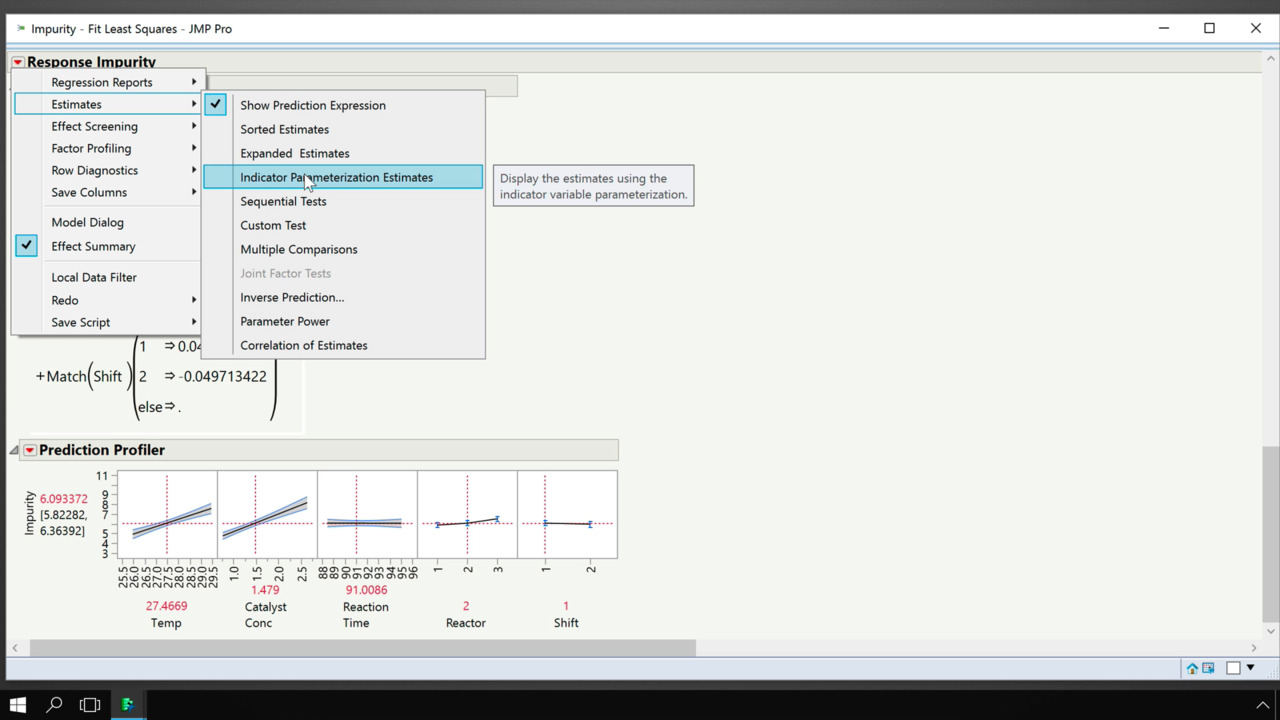
It’s important to note that these two coding schemes result in the same model predictions. But, from an explanatory perspective, the interpretation of the coefficients is different. Let’s turn our attention to the variable Reactor, which has three levels. In this case, the regression model includes two indicator variables, with coefficients for Reactor 1 and Reactor 2. Again, we can apply either effect coding or dummy coding.
Here, effect coding is applied:
- Reactor number 1 is coded as 1 for Reactor[1] and 0 for Reactor [2].
- Reactor number 2 is coded as 0 for Reactor[1] and 1 for Reactor [2].
- Reactor number 3 is coded as -1 for Reactor[1] and -1 for Reactor [2].
The average of Impurity for Reactor 1 is 0.82 below the average, and the average of Impurity for Reactor 2 is 0.42 below the average.
Why don’t we report a coefficient for Reactor 3? It turns out that, for three-level categorical predictors, the last level is redundant to the first two levels.
The interpretation for effect-coded estimates is that each coefficient is the difference from the average. Because these coefficients must sum to zero, the average of Impurity for Reactor 3 can easily be calculated from the first two: the average of Impurity for Reactor 3 is 1.24 above the average.
As a generalization, for a k-level categorical predictor, the software computes k-1 coefficients.
Let's return to our model results. The p-values for the whole model and the parameter estimates are very low, indicating that there are significant differences in the average Impurity for the different reactors.
Now, we'll put it all together. We fit a model for Impurity with all five predictors. Again, the p-value in the ANOVA table indicates that the whole model is significant.
The Effect Summary table provides tests for the whole effects. We see that Temp, Catalyst Conc, and Reactor are all significant, adjusting for the other terms in the model.
As a reminder, here are the results for our model with only the three continuous predictors.
Root Mean Square Error for our new model is lower. And RSquare for our new model is higher. So, more of the variation in Impurity is explained by our model.
However, RSquare can be inflated by adding more terms to the model, even if these new terms are not significant. So, in multiple linear regression situations, we use RSquare Adjusted when comparing different models with the same data instead of using RSquare. RSquare Adjusted applies a penalty for each additional term, p, that is added to the model. If a term is added to the model that does not explain variation in the response, RSquare Adjusted goes down.
RSquare Adjusted for our new model is higher than RSquare Adjusted for our original model. This confirms that the new model fits better than the original model.
But can we do better? Are there other terms we can add to the model? We explore this in an upcoming section.