Example of a Gaussian Process Model
Given a specified engineering model, use a Gaussian process model to understand the impact of factors included in the model on the response. The data demonstrate the flow of water through a Borehole that is drilled from the ground surface through two aquifers.
1. Select Help > Sample Data Folder and open Design Experiment/Borehole Latin Hypercube.jmp.
2. Select Analyze > Specialized Modeling > Gaussian Process.
3. Select log10 Rw through Kw and click X.
4. Select Y and click Y.
5.  In JMP Pro, to run the analysis faster, leave the Fast GASP checked.
6. Click OK.
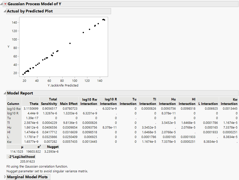
Figure 17.5 Borehole Latin Hypercube Report
Note: The estimated parameters can be different due to different starting points in the minimization routine or different fitting options. The results shown above were obtained using the Fast GASP routine in JMP Pro.
The data on the actual by predicted plot fall along the Y = X line, indicating that the Gaussian process prediction model is a good approximation of the true function. In the Model Report, you see that the first factor, log10 Rw, has the highest total sensitivity. The estimated total sensitivity for log10 Rw explains more than 90% of the variation in the response. Factors with small theta values have little (or no) impact on the prediction formula. Use the profiler to visualize the sensitivities.
7. Click the Gaussian Process Model of Y red triangle and select Profiler.
The desirability functions automatically appear because the response, Y, has a Response Limits column property.
8. Click the Prediction Profiler red triangle and select Optimize and Desirability > Maximize Desirability. Adjust the Y axis, if needed, to view the optimal results.
Figure 17.6 Gaussian Process Model Profiler
The desirability function is set to maximize the response Y because Y has goal set to Maximize in the Response Limits column property. Maximizing the desirability functions identifies the values of the factors that maximize the response. The shaded bands represent the 95% confidence intervals.

