Example of Examining the Residuals in a Loglinear Variance Model
After fitting a loglinear variance model, you can analyze the residuals by saving the residuals to the data table.
1. Select Help > Sample Data Folder and open InjectionMolding.jmp.
2. Select Analyze > Fit Model.
Since the variables in the data table have been assigned preselected roles, the analysis runs automatically.
3. Click the Loglinear Variance Fit red triangle and select Save Columns > Residuals.
4. In the InjectionMolding.jmp sample data table, right-click the continuous icon next to Hold Time in the Columns panel, and select Nominal.
5. Select Analyze > Fit Y by X.
6. Select Shrinkage Residual and click Y, Response.
7. Select Hold Time and click X, Factor.
8. Click OK.
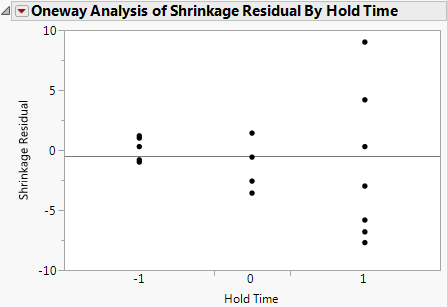
Figure 11.6 Residual by Dispersion Effect
In this plot it is easy to see the variance go up as the Hold Time increases. This is done by treating Hold Time as a nominal factor.
