Example of Maximum Likelihood
This example uses the Nonlinear platform to minimize a loss function. The loss function is the negative of a log-likelihood function, thus producing maximum likelihood estimates.
Estimate the Model
1. Select Help > Sample Data Folder and open Nonlinear Examples/Logistic w Loss.jmp.
2. Select Analyze > Specialized Modeling > Nonlinear.
3. Assign Model Y to the X, Predictor Formula role.
This column contains the linear model. The model is shown in the Predictor section of the launch window.
4. Assign Loss to the Loss role to define a custom loss function.
Figure 15.12 Nonlinear Launch Window
5. Click OK.
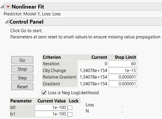
Figure 15.13 Nonlinear Fit Control Panel
6. Click Go in the Control Panel.
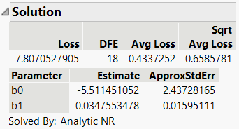
Figure 15.14 Solution Report
The Loss value in the Solution report is the negative log-likelihood evaluated at the parameter estimates.
Create Custom Profiler
Because our model was fit using a custom loss function, a standard profiler is not available. Use the custom profiler to explore model predictions.
1. Click the Nonlinear Fit red triangle and select Custom Estimation Profiler.
2. Enter the model as the custom estimation expression. To do so enter the following expression in the Enter Expression window:
1/(1 + Exp( b0 + b1*x ))
3. Select Logit from the Transformation list.
Figure 15.15 Completed Enter Expression Window
4. Click OK.
5. Enter 100 as the initial value.
6. Click OK.
By default, the profiler is difficult to interpret because the ranges for response and the factor are narrow. You can adjust the axis settings to use a meaningful range.
7. Double click the vertical axis. In the Scale outline, specify 0 as the Minimum and 1 as the Maximum.
8. Click OK.
9. Double click the horizontal axis. In the Scale outline, specify -100 as the Minimum and 400 as the Maximum.
10. Click OK.
Figure 15.16 Custom Estimation Profiler
The custom profiler shown is titled by the custom expression and shows the value of the response across the values of the x variable. The profiler also displays the 95% confidence intervals.


