Statistical Details for Distance Measures
This section contains statistical details for the distance measures used in the Outlier Analysis plots in the Multivariate platform.
Mahalanobis Distance Measures
The Mahalanobis distance takes into account the correlation structure of the data and the individual scales. For each value, the Mahalanobis distance is denoted Mi and is computed as follows:

where:
Yi is the data for the ith row
 is the row of means
S is the estimated covariance matrix for the data
The UCL reference line (Mason and Young 2002) drawn on the Mahalanobis Distances plot is computed as follows:
UCLMahalanobis = 
where:
n = number of observations
p = number of variables (columns)
 = (1–α)th quantile of a Beta
  distribution
If a variable is an exact linear combination of other variables, then the correlation matrix is singular and the row and the column for that variable are zeroed out. The generalized inverse that results is still valid for forming the distances.
Jackknife Distance Measures
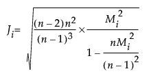
The jackknife distance is calculated with estimates of the mean, standard deviation, and correlation matrix that do not include the observation itself. For each value, the jackknife distance is computed as follows:

where:
n = number of observations
p = number of variables (columns)
Mi = Mahalanobis distance for the ith observation
The UCL reference line (Penny 1996) drawn on the Jackknife Distances plot is calculated as follows:

T2 Distance Measures
The T2 distance is the square of the Mahalanobis distance, so Ti2 = Mi2.
The UCL on the T2 distance is:

where
n = number of observations
p = number of variables (columns)
 = (1–α)th quantile of a Beta
  distribution
Multivariate distances are useful for spotting outliers in many dimensions. However, if the variables are highly correlated in a multivariate sense, then a point can be seen as an outlier in multivariate space without looking unusual along any subset of dimensions. In other words, when the values are correlated, it is possible for a point to be unremarkable when seen along one or two axes but still be an outlier by violating the correlation.