Statistical Details for the Fit Orthogonal Option
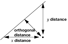
In the Bivariate platform, you can use the Fit Orthogonal option to fit a line that minimizes the sum of the squared perpendicular differences. This can be preferable to standard least squares when there is random variation in the measurement of X. Standard least square fitting assumes that the X variable is fixed and the Y variable is a function of X plus error.
Note: The perpendicular distance depends on how X and Y are scaled, and the scaling for the perpendicular is reserved as a statistical issue, not a graphical one.
Figure 5.22 Line Perpendicular to the Line of Fit
The fit requires that you specify the ratio of the variance of the error in Y to the error in X. This is the variance of the error, not the variance of the sample points, so you must choose carefully. In standard least squares, the ratio  is infinite because
  is zero. An orthogonal fit with a large error ratio approaches the standard least squares line of fit. If you specify a ratio of zero, the fit is equivalent to the regression of X on Y, instead of Y on X.
The most common use of this technique is in comparing two measurement systems that both have errors in measuring the same value. Thus, the Y response error and the X measurement error are both the same type of measurement error. The error ratio is an assumed value, such as 1 (equal variances), or can be based on knowledge of the measurement systems.
Confidence limits are calculated as described in Tan and Iglewicz (1999).
