Additional Example of Support Vector Machines
In this example, you use Support Vector Regression (SVR) to model a continuous response. SVR models use the SVM algorithm to predict continuous response data. Use the same medical data on patients who have diabetes that was used in Example of Support Vector Machines. However, instead of a binary measure of diabetes disease progression, you now have a continuous measure. Higher values correspond to more disease progression. Vary the cost parameter of the radial basis function to find the best fitting model.
1. Select Help > Sample Data Folder and open Diabetes.jmp.
2. Select Analyze > Predictive Modeling > Support Vector Machines.
3. Select Y and click Y, Response.
4. Select Age through Glucose and click X, Factor.
5. Select Validation and click Validation.
6. Click OK.
7. In the Model Launch control panel, check that the kernel function is a Radial Basis Function with Cost parameter 1 and Gamma parameter 0.1.
8. Click Go.
9. Click the gray triangle next to Model Launch to open the Model Launch control panel.
10. Change the cost parameter to 0.1.
11. Click Go.
12. Click the gray triangle next to Model Launch to open the Model Launch control panel.
13. Change the cost parameter to 2.
14. Click Go.
Figure 9.6 Model Comparison Report
The Model Comparison report contains the results of the models using different cost parameters. Recall that a higher cost parameter implements an algorithm that is less likely to misclassify a point, whereas a lower cost parameter implements a more flexible algorithm. In this scenario, the more flexible model (cost parameter equal to 0.1) produces the best model fit.
15. In the Show column of the Model Comparison report, deselect Model 1 and Model 3.
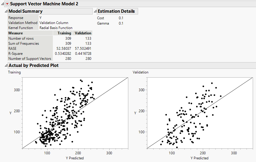
Figure 9.7 Model Report for Continuous Response
The model report for a continuous response contains the Model Summary, Estimation Details, and Actual by Predicted Plot. In the Model Summary report, the RASE is 52.58 for the training set and 57.50 for the validation set.

