Example Comparing Split Plot Designs
Use the Compare Design platform to compare two split-plot designs with different numbers of whole plots. The designs are for three factors:
• A continuous hard-to-change factor
• A continuous easy-to-change factor
• A three-level categorical easy-to-change factor
The designs include all two-factor interactions in the assumed model. You can afford 20 runs and want to compare using 4 or 8 whole plots.
Launch Compare Designs
1. Select Help > Sample Index, click the Sample Index red triangle and select Open Sample > Script. Open Compare Split Plots.jsl.
2. Right-click in the script window and select Run Script.
Two design tables are constructed using Custom Design:
– 4 Whole Plots
– 8 Whole Plots
You want to compare these two designs. Notice that the 4 Whole Plots table is active.
3. In the 4 Whole Plots table, select DOE > Design Diagnostics > Compare Designs.
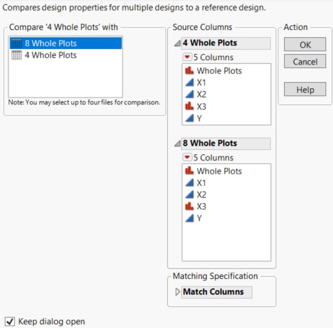
4. From the Compare ‘4 Whole Plots’ with list, select 8 Whole Plots.
A panel for this design is added to the launch window. JMP automatically matches the columns in the order in which they appear in the two design tables.
Figure 17.27 Completed Launch Window
5. Click OK.
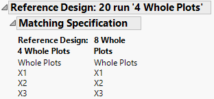
6. Open the Matching Specification section under Reference Design: 20 run ‘4 Whole Plots’.
Figure 17.28 Matching Specification for Split-Plot Designs
Notice that the Whole Plots column is entered as part of the design. This is necessary because Compare Designs needs to know the whole plot structure.
Examine the Report
The Design Evaluation report provides various diagnostics that compare the two designs.
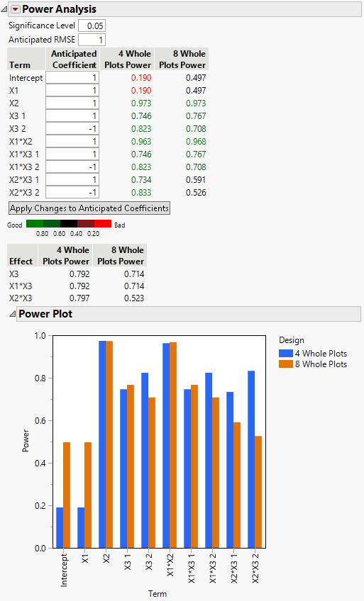
Figure 17.29 Power Analysis for Two Split-Plot Designs
The Power Analysis report shows that the power for the whole-plot factor, X1, is much smaller for the four whole-plot design (0.19) than for the eight whole-plot design (0.497). However, the four whole-plot design has higher power to detect split-plot effects, especially the interaction of the two split-plot factors, X2*X3 (0.797 compared to 0.523). Notice that the power for the combined effect X2*X3 is given under the color bar and legend.
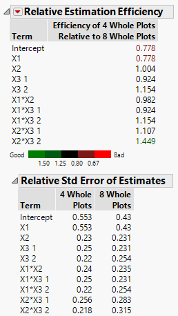
Figure 17.30 Relative Estimation Efficiency Comparing Split-Plot Designs
The Relative Estimation Efficiency report shows the relative estimation efficiency for X1 to be 0.778. This indicates that the standard error for X1 is notably larger for the four whole-plot design than for the eight whole-plot design.
Open the Relative Std Error of Estimates report. You can see that the relative standard error for X1 in the four whole-plot design is 0.553, compared to the eight whole-plot error of 0.43.
In the Relative Estimation Efficiency report, the relative estimation efficiency for X2*X3 2 is 1.449, indicating that the standard error for the parameter associated with X2*X3 2 is notably larger for the eight whole-plot design than for the four whole-plot design.
The Power Analysis and the Relative Estimation Efficiency reports indicate that the choice of designs revolves around the importance of detecting the whole plot effect X1. The eight whole-plots design gives you a better chance of detecting a whole plot effect. The four whole-plots design is somewhat better for detecting split-plot effects involving the categorical variable.


