Example of a Latent Growth Curve Model
Latent growth curve (LGC) models enable analysts to model longitudinal data and characterize trajectories over time. The most common latent growth curve model is one of linear growth, where intercept and slope latent variables are specified to capture the overall trajectory of the process and individual observations’ deviations from the overall trajectory. This model is very similar to a random coefficients model. A key feature of LGC models is that they place constraints on the mean structure of the data. Modeling the mean structure enables you to test hypotheses related to growth.
In this example, you are modeling the achievement scores of students over 4 years of an academic program using a multiple choice test score. You want to test the hypothesis that a linear trajectory characterizes this process.
1. Select Help > Sample Data Folder and open Academic Achievement.jmp.
2. Select Analyze > Multivariate Methods > Structural Equation Models.
3. Select Multiple Choice Year1 through Multiple Choice Year4 and click Model Variables.
4. Click OK.
The Structural Equation Models report Model Specification outline appears.
5. Select Model Shortcuts > Longitudinal Analysis > Linear Latent Growth Curve.
The Model Specification diagram now shows a linear latent growth curve model.
6. Click the Lists tab in the View panel box.
7. Select the first 4 items in the Variances list and click Set Equal.
This constrains the residual variances for each variable to be equal, which is analogous to a homogeneity of variance assumption. In SEM, this assumption is testable, such that another model can be fit without equality constraints and compared with a chi-square difference test.
8. In the text box below Model Name, type Linear LGC with Equal Variances.
9. Click Run.
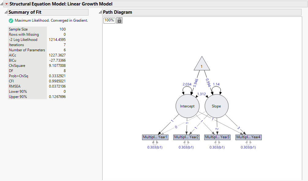
Figure 8.11 Summary of Fit and Path Diagram for Linear LGC Model
The chi-square statistic for this model, listed in the Summary of Fit report, is 9.11 with 8 degrees of freedom. Note that the corresponding p-value is 0.3333, which is not significant. This indicates that there is not evidence to reject the null hypothesis that the model fits well. Therefore, you conclude that this model fits the data reasonably well. The CFI and RMSEA fit indices also indicate excellent fit as they are greater than 0.9 and less than 0.1, respectively.
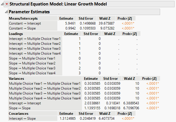
Figure 8.12 Parameter Estimates for Linear LGC Model
The mean estimate of the intercept is 5.95, which indicates the overall achievement score at year 1. This means that, on average, students’ academic achievement is 5.96 on the first occasion of measurement. The mean of the intercept is centered at the first occasion because the slope factor has a zero loading on that variable.
The mean estimate of the slope is 0.99, which indicates that the overall achievement scores increase by 0.99 each year. The significant variance estimates of the intercept and slope factors point to significant variability around the average trajectory; not everyone starts at the same place and not everyone increases at the same rate. External variables can be used as predictors of the intercept and slope to understand what leads to differences in the trajectories of individuals.
Lastly, the positive covariance between intercept and slope suggests that those who start with higher levels of academic achievement on the first year tend to increase more rapidly over time.
LGC models provide a flexible approach for investigating how processes change over time. The Model Shortcuts menu provides alternative trajectories that can be fit and tested against each other to ascertain the best model fit, including a no-growth trajectory, a quadratic trajectory, and even a non-linear trajectory with the Latent Basis option.

