Example of Confidence and Prediction Intervals Using Formulas
In this example, use the Prediction and Interval Formulas option from a standard least squares model to create a prediction profiler with confidence and prediction intervals.
Fit the Model
Fit a standard least squares regression model using data on diabetes patients.
1. Select Help > Sample Data Folder and open Diabetes.jmp.
2. Select Analyze > Fit Model.
3. Select Y and click Y.
By default, the Personality is set to Standard Least Squares.
4. Select Age through Total Cholesterol and click Add.
5. Select Validation and click Validation.
6. Click Run.
7. Click the Response Y red triangle and select Save Columns > Prediction and Interval Formulas.
Launch the Profiler
The data table now contains a prediction column named Pred Formula Y and several hidden columns. The hidden columns contain formulas for the confidence limits and prediction limits. These formula columns are used automatically in the Profiler platform.
1. Select Graph > Profiler.
2. Select Pred Formula Y and click Y, Prediction Formula.
3. Click OK.
4. Click the Prediction Profiler red triangle and select Prediction Intervals.
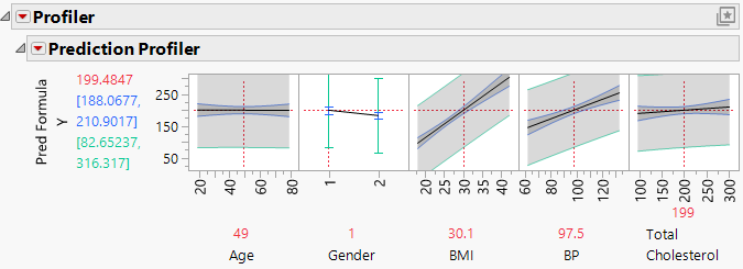
Figure 3.39 Profiler with Confidence and Prediction Intervals
A prediction profiler is shown with confidence and prediction intervals constructed using the limits in the hidden columns. The confidence intervals are shown in blue, and the prediction intervals are shown in green. Since the prediction intervals are for an individual observation, they include more variation and are wider than the confidence intervals.
