Example of Design Space Profiler
Use the Design Space Profiler option in the Prediction Profiler to find operational ranges for three factors that predict an in-spec response at least 75% of the time.
1. Select Help > Sample Data Folder and open Tiretread.jmp.
2. Select Graph > Profiler.
3. Select Pred Formula MODULUS and click Y, Prediction Formula.
4. Click OK.
5. Click the Prediction Profiler red triangle and select Design Space Profiler.
6. In the Enter Spec Limits window, specify 1000 as the lower specification limit (LSL) and 2000 as the upper specification limit (USL). These are the specification limits for Modulus.
7. Click OK.
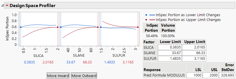
Figure 3.40 Initial Design Space Profiler Report
The initial Design Space Profiler report shows a profiler graph for each factor and several tables. With the factors unconstrained over their full ranges, the InSpec Portion is 58.48%. This means that without defining an operating range, the factors predict responses that fall between 1000 and 2000 about 58% of the time. Now explore setting operating limits on the factors.
8. Click Move Inward.
The first specification limit to move is the LSL of SILANE.
9. Click Move Inward until the InSpec Portion is above 0.75.
Note: This should take a total of about 11 clicks.
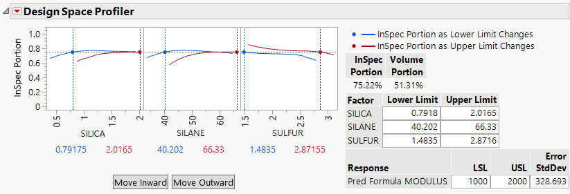
Figure 3.41 Updated Design Space Profiler
The updated Design Space Profiler report shows that setting operating limits improves the InSpec Portion to about 75%. The factor SULFUR keeps a relatively wide range, with only its USL moving slightly inward. The other factors, SILICA and SILANE, keep their USLs at their respective maximums while their LSLs moved inward.
10. Click the Design Space Profiler red triangle and select Make and Connect Random Table.
11. In the Output Random Table window, deselect Add Random Noise.
12. In the Output Random Table window, select Embed Factor Space Scatterplots.
13. Click OK in the Output Random Table window.
The data table contains 10,000 rows of uniformly distributed factor settings with their corresponding simulated responses.
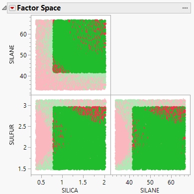
Figure 3.42 Scatterplot Matrix Highlighting Desirable Operating Space
The scatterplots provide a visual representation of the operating limits and their impact on the in spec results. Predicted responses that are within the specification limits are colored green and predicted responses that are outside of the specification limits are colored red. The selected points contain factors at values that are within the operating limits.


