 Example of K Nearest Neighbors with a Categorical Response
In this example, you want to construct a model to classify the credit risk of customers who apply for home equity loans. You have historical financial data for 5,960 customers where each customer was classified as being a Good Risk or Bad Risk. There are missing values for many of the predictors.
1. Select Help > Sample Data Folder and open Equity.jmp.
2. Select Analyze > Predictive Modeling > K Nearest Neighbors.
3. Select BAD and click Y, Response.
4. Select LOAN through CLNO and click X, Factor.
Because one of the potential predictors, DEBTINC, has many missing values, you do not include it in your model. Missing values for continuous predictors are replaced by the average of the predictor. This procedure sometimes works well for values that are missing at random. Although the high missing rate of the DEBINC indicates that the missing might be informative, we do not investigate that in this example.
5. Select Validation and click Validation.
6. Click OK.
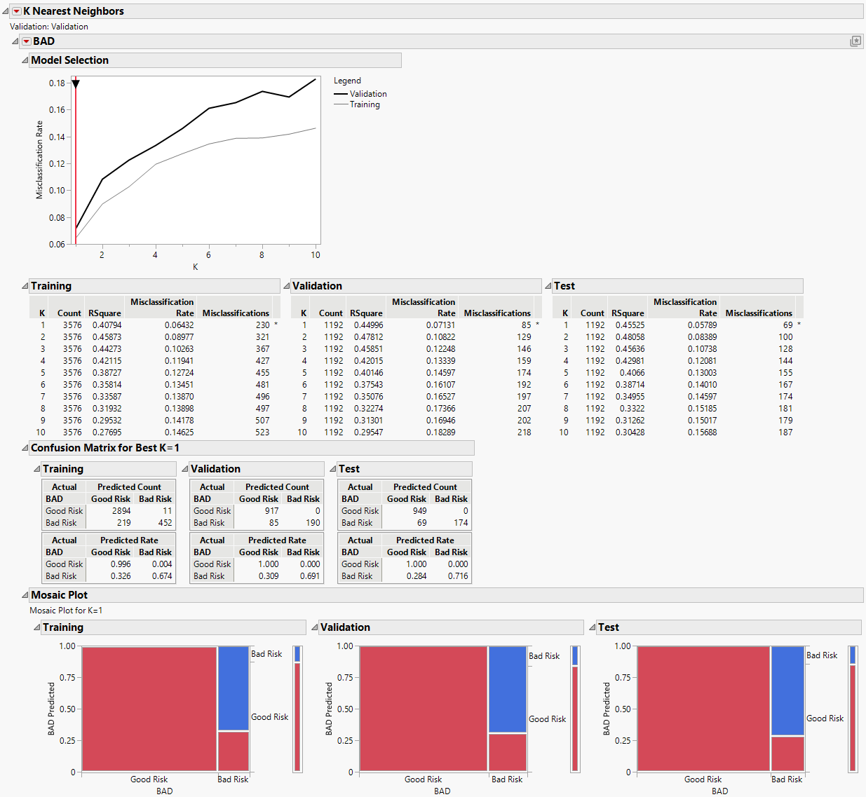
Figure 7.2 K Nearest Neighbors Report
For each value of K, JMP constructs a model using only the training set observations. Each of these models is used to classify the validation set observations. The validation set results are used to select a best model. In this example, the model based on the single nearest neighbor (K = 1) has the smallest misclassification rate. The test set verifies that the single nearest neighbor model is the best performer for independent data.
7. Click the BAD red triangle and select Publish Prediction Formula.
8. Next to Number of Neighbors, K, leave the default value of 1.
9. Click OK.
The prediction equation is saved in the Formula Depot. You can compare the performance of alternative models published to the Formula Depot with that of the K = 1 nearest neighbor model using the Model Comparison option in the Formula Depot. See “Formula Depot”.
