Example of Two-Way Analysis of Variance
Use the Standard Least Squares personality of the Fit Model platform to fit a two-way analysis of variance model. You then use the model to explore predictions based on settings of the variables.
1. Select Help > Sample Data Folder and open Analgesics.jmp.
2. Select Analyze > Fit Model.
3. Select pain and click Y.
4. Select gender and drug and click Add.
5. Click Run.
6. Click the Response pain red triangle menu and select Factor Profiling > Profiler.
Report sections are shown and described below.
Leverage Plots
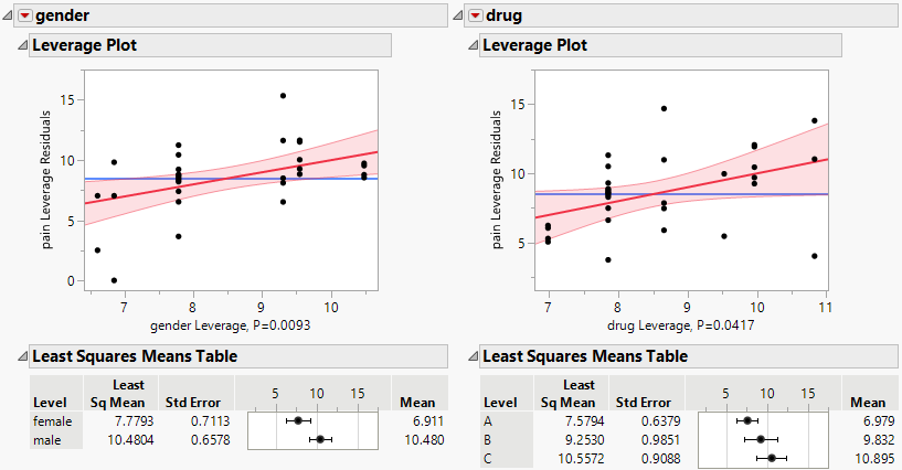
Use the leverage plots to identify influential observations and assess their impact on the regression model.
Figure 4.8 Leverage Plot and Least Squares Means Table for Factors
You do not observe any highly influential points. You do observe that both gender and drug have some impact on the response based on the upward trend of the fitted lines and the least squares means values that shift with the levels of gender and drug.
Actual by Predicted Plot
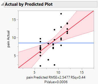
Use the Actual by Predicted Plot to assess the performance and accuracy of the model by comparing the actual values of the pain response with the predicted values from the model.
Figure 4.9 Actual by Predicted Plot
The plot and p-value of 0.0006 indicate that the relationship between the actual and predicted values is statistically significant.
Model Fit Summary Tables and Residual Plot
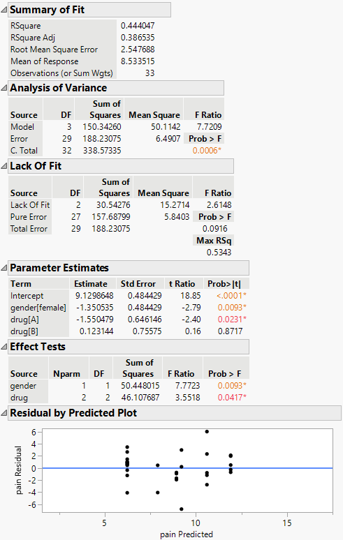
Use the tables in the report to assess model fit and response variable statistics. The Summary of Fit table contains information to assess model fit and response variable statistics. The Analysis of Variance table contains information about the overall model significance and sources of variation. The Lack of Fit table contains information about model adequacy and error assessment. The Parameter Estimates table contains coefficients, standard errors, and predictor significance. The Effect Tests table contains information about the significance of individual predictors. The Residual by Predicted Plot is to evaluate the assumptions and performance of the regression model by examining the patterns or trends in the residuals across the range of predicted values.
Figure 4.10 Model Summary with ANOVA, Parameters, and Residuals
The tables indicate a regression model with an R-square statistic of 0.444. The effect tests for gender and drughow both factors are statistically significant (with a p-value < 0.05).
Prediction Profiler
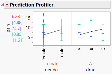
Use the Prediction Profiler to explore how the predicted value of the response varies based on the predictor settings.
Figure 4.11 Prediction Profiler
The predicted pain response is 6.23 with a 95% confidence interval of 4.88 to 7.57 for females who took type A of the drug. You can interactively explore the response for various combinations of gender and drug levels in the Prediction Profiler. To visualize how the pain response varies across different combinations of the factor levels, click on the desired level of either gender or drug and then click on the levels of the other factor.
Tip: To fit a prediction interval, use the Prediction Interval option in the Prediction Profiler red triangle menu. Prediction intervals are wider than confidence intervals. Prediction intervals are for a new observation not used in the construction of the model.


