Transcendental Functions
In the JMP Formula Editor, you can create a formula that supports transcendental functions, such as logarithmic functions for any base, functions for combinatorial calculations, the Beta function, and several gamma functions. See “Transcendental Functions” in the Scripting Guide for more information about syntax.
Exp
Raises e to the power that you specify. Thus, Exp(1) = e.
ExpM1
Returns a more accurate calculation of Exp(x) - 1 when x is very small.
Ln
Calculates the natural logarithm of x.
Log and Log10
Calculates the natural logarithm (base e). To change the default base, highlight the argument and type a comma or click the Insert key on the Formula Editor keypad. The base appears and is editable. The Log argument can be any numeric expressions. The expression Log(e) evaluates as 1, and Log(32,2) is 5. The Log10 function calculates the logarithm of base 10 only.
Log1P
Returns a more accurate calculation of Log(1+x) when x is very small.
Squash
Computes the function 1 / (1 + ex), where x is any numeric column, variable, or expression.
Logist
Also known as Squish or Logistic, is an efficient computation of the function 1 / (1+e-x), where x is any numeric column, variable, or expression.
Root (Square Root)
Calculates the root of its argument as specified by the index. Root initially shows with an index of 2. To change the index, highlight the index argument and enter the value that you want.
Factorial
Returns the product of all numbers 1 through the argument that you specify. For example, Factorial(5) evaluates as 120.
NChooseK
Returns the number of n things taken k at a time (n select k) and is computed in the standard way using factorials, as n! / (k!(n – k)!). For example, NChooseK(5,2) evaluates as 10.
Beta
Adds the two parameter Beta function and is written terms of the Gamma function as:

Gamma
Adds the Gamma function, denoted Γ(i), and is defined as:

Gamma with a single argument is the same as Gamma(x, infinity). The optional second argument changes the upper integer from infinity to the value that you enter. Other interesting gamma function relationships are
• for any α > 1, Γ(α) = (α–1) • Γ(α–1)
• for any positive integer, n, Γ(n) = (n-1)!
• Γ(0.5) = the square root of π
LGamma
Is the natural log of the result of the gamma function evaluation. You get the same result using the Log (natural log) function with the Gamma function. However, the LGamma function computes more efficiently than do the Log (natural log) and the Gamma functions together. NChooseK is implemented using LGamma functions. The result is not always an exact integer. If the result is close to an integer, it is rounded up using the Floor function.
Digamma
The logarithmic derivative of the Gamma function.
Trigamma
The derivative of the Digamma function, or the logarithmic second derivative of the Gamma function.
Arrhenius
Calculates the non-specific component of the Arrhenius relationship that is then multiplied by the activation energy in the Arrhenius equation.

Arrhenius Inv
The inverse of the Arrhenius function:

Logit
Applies the logit transformation to the argument using:

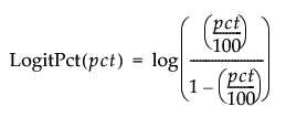
Logit Percent
Calculates the logit as a percent for the argument.

Logist Percent
Calculates the logistic as a percent for the argument.

Scheffe Cubic
Is used in fitting certain models. Scheffe Cubic (X1, X2) is equivalent to X1*X2*(X1-X2).
SbInv
Johnson Sb inverse transformation. If argument is normal, the result is Johnson Sb.
SbTrans
Johnson Sb transformation from a doubly bound variable to a standard normal (0, 1) distribution.
SHASHInv
Returns a transformation of a standard normal variable into a sinh-arcsinh (SHASH) distributed variable.
SHASHTrans
Returns a transformation of a sinh-arcsinh (SHASH) distributed variable into a standard normal distributed variable.
SlInv
Johnson Sl inverse transformation. If argument is normal, the result is Johnson Sl.
SlTrans
Johnson Sl transformation from a doubly bound variable to a standard normal (0, 1) distribution.
SuInv
Johnson Su inverse transformation. If argument is normal, the result is Johnson Su.
SuTrans
Johnson Su transformation from a doubly bound variable to a standard normal (0, 1) distribution.