 Example of a Gaussian Process Model with Categorical Predictors
Predict the response using a Gaussian Process model that contains both continuous and categorical factors. These data are simulated CPU times from a 50 run space filling designed experiment that has three continuous and two categorical factors.
1. Select Help > Sample Data Folder and open Design Experiment/Algorithm Data.jmp.
2. Select Analyze > Specialized Modeling > Gaussian Process.
3. Select Alpha through Compiler and click X.
4. Select CPU Time and click Y.
5.  To run the analysis, leave the Fast GASP checked. Click OK.
Note: The Fast GASP option must be used for models that contain categorical factors. See Statistical Details for Models with Categorical Predictors.
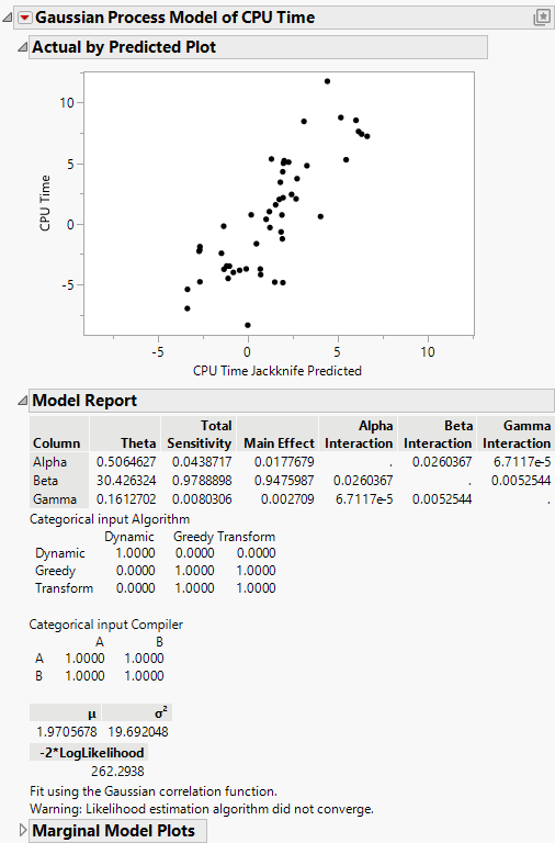
Figure 17.7 Algorithm Data Report
Note: The estimated parameters can be different due to different starting points in the minimization routine.
The actual by predicted plot shows a strong correlation between the actual and predicted CPU times. This in an indication that the Gaussian process prediction model is a good approximation of the true function. In the Model Report, the Beta predictor has the highest total sensitivity. This indicates that of the continuous predictors, Beta explains the most variation in the response. There is a separate Categorical Input matrix for each of the categorical predictors, Algorithm and Compiler. These matrices are correlation matrices and show the correlation between levels for each categorical predictor. The off-diagonals of the matrices are the τ parameters.
