Example of a Polynomial Effects Model
Use the Standard Least Squares personality of the Fit Model platform to fit a cubic polynomial model to bivariate data.
1. Select Help > Sample Data Folder and open Growth.jmp.
2. Select Analyze > Fit Model.
3. Select ratio and click Y.
4. Type 3 in the text box next to Degree.
5. Select age and click Macros > Polynomial to Degree.
This adds three terms to the models.
6. Click Run.
The report sections are shown and described below.
Leverage Plots
Use the leverage plots to identify influential observations and assess their impact on the regression model.
Figure 4.2 Leverage Plots
The leverage plots show no influential data points and that all the variables in the model are significant.
Regression and Actual by Predicted Plots
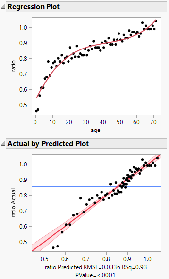
Use the Regression and Actual by Predicted Plots to assess the performance and accuracy of the model.
Figure 4.3 Regression and Actual by Predicted Plots
The Regression Plot shows the data points with the nonlinear (cubic polynomial) regression model fit to the data. The points in the Actual by Predicted Plot follow the y = x line, which suggests that the model predictions are close to the actual values.
Model Fit Summary Tables and Residual Plot
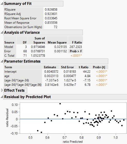
Use the tables in the report to assess model fit and response variable statistics. The Summary of Fit table contains information to assess model fit and response variable statistics. The Analysis of Variance table contains information about the overall model significance and sources of variation. The Parameter Estimates table contains coefficients, standard errors, and predictor significance. The Effect Tests table contains information about the significance of individual predictors. The Residual by Predicted Plot is to evaluate the assumptions and performance of the regression model by examining the patterns or trends in the residuals across the range of predicted values.
Figure 4.4 Regression Model Summary and Residual Analysis
In this example, the Analysis of Variance and Parameter Estimates tables indicate that the model is statistically significant and that all of the coefficients for the variables included in the model are statistically significant, respectively. Also, the Summary of Fit table shows a high R-square value of 0.927, which indicates a strong relationship between the predictors and the response variable.
The Residual by Predicted Plot shows that the residuals are randomly scattered and evenly distributed above and below the zero line. This suggests that the model assumptions are met and the residuals are normally distributed.


