Example of a Response Surface Model
Use the Standard Least Squares personality of the Fit Model platform to fit a response surface model. Your objective is to minimize the response.
Fit the Full Response Surface Model
1. Select Help > Sample Data Folder and open Design Experiment/Custom RSM.jmp.
2. Select Analyze > Fit Model.
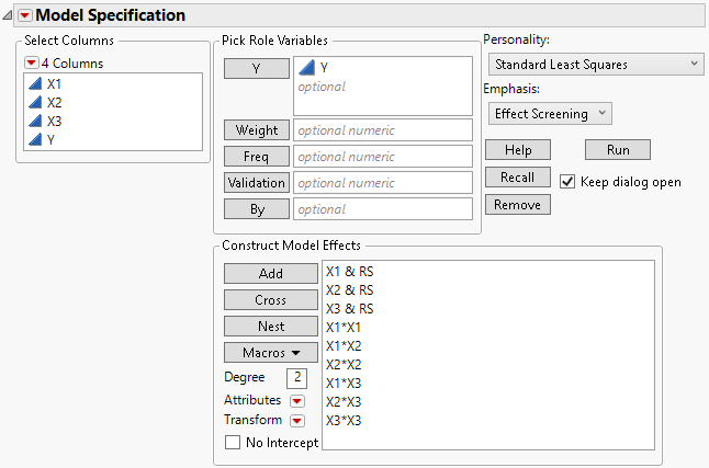
Because the data table contains a Model script, the Model Specification window is filled out as specified in the Model script. Note the following:
– Main effects appear in the Construct Model Effects list with a &RS suffix, which indicates that the Response Surface macro has been applied.
– The effects are those for a full response surface in the three predictors X1, X2, and X3.
– Because the model contains terms with the &RS suffix, the analysis results include a Response Surface report.
Figure 4.26 Fit Model Launch Window for the Response Surface Analysis
3. Click Run.
Reduce the Model
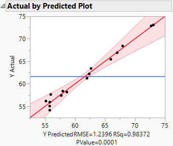
The Actual by Predicted Plot shows that the model is useful. From the Lack of Fit table (not shown), there is no evidence of lack of fit.
Figure 4.27 Actual by Predicted Plot for Full Model
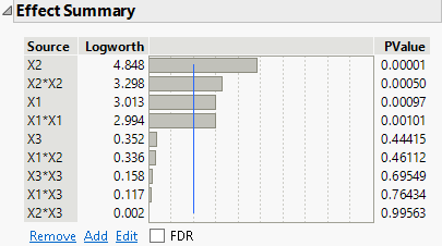
The Effect Summary report suggests that a number of effects are not significant. In particular, X2*X3 is the least significant effect with a p-value of 0.99563. Use the controls in the Effects Summary Report to reduce the model.
Figure 4.28 Effect Summary Report
1. In the Effect Summary report, click X2*X3 and click Remove.
The model updates.
The PValue column in the Effect Summary report indicates that X1*X3 is not significant.
2. Click X1*X3 and click Remove.
The p-value for X3*X3 indicates that it is not significant.
3. Click X3*X3 and click Remove.
4. Click X1*X2 and click Remove.
Notice that X3 is not significant. It is not contained in any higher-order effects, so you can remove it without violating the Effect Heredity principle. See “Effect Heredity”.
5. Click X3 and click Remove.
Figure 4.29 Effect Summary Report After Reducing Model
All remaining effects are significant, which indicates that their coefficients in the model are different from zero.
Examine the Response Surface Report
1. Click the Response Y red triangle and select Estimates > Show Prediction Expression.
Figure 4.30 Prediction Expression
Tip: The Prediction Expression is the prediction formula. You can also obtain this formula by selecting Save Columns > Prediction Formula.
In the following steps, you can refer to the prediction expression to see the model coefficients.
2. Open the Response Surface report and then the Canonical Curvature report.
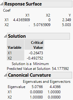
Figure 4.31 Response Surface Report
The first table gives the second-order model coefficients in matrix form. The coefficient of X1*X1 is 4.4365909, the coefficient of X2*X2 is 5.0765909, and the coefficient of X1*X2 is 0. The coefficients of the linear effects, 2.349 for X1 and 5.003 for X2, are given in the column labeled Y.
The Solution report shows the critical values. These are the values where a maximum, a minimum, or a saddle point occur. In this example, the Solution report indicates that the response surface achieves a minimum of 54.18 at the critical value, where X1 = -0.265 and X2 = -0.493.
The Canonical Curvature report shows the eigenstructure of the matrix of second-order parameter estimates. The eigenstructure is useful for identifying the shape and orientation of the curvature. See “Canonical Curvature Report”.
In this example, both eigenvalues are positive, which indicates that the surface achieves a minimum. The direction of greatest curvature corresponds to the largest eigenvalue (5.0766). That direction is defined by the corresponding eigenvector components. For the first direction, X2, with an eigenvector value of 1.00, determines the direction. The second direction is determined by X1, also with an eigenvector value of 1.00.
Find the Critical Point Using the Prediction Profiler
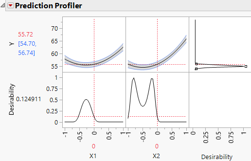
The Prediction Profiler report shows the quadratic behavior of the response surface along traces for X1 and X2. Because the Response Limits column property is set for Y, the profiler also shows desirability functions.
Figure 4.32 Prediction Profiler with Match Target as Goal
The goal for the Response Limits column property is set to Match Target. For this example, you are interested in minimizing Y, not matching a target. Therefore, you must change the setting:
1. Press Ctrl and click in the top right cell of the Prediction Profiler.
2. In the Response Goal window, select Minimize from the list of options.
3. Click OK.
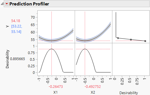
The desirability function now reflects your goal of minimizing Y.
4. Click the Prediction Profiler red triangle and select Optimization and Desirability > Maximize Desirability.
Figure 4.33 Prediction Profiler with Minimize as Goal and Desirability Maximized
Settings within the design region that minimize Y appear under the profiler. Note that these are precisely the Critical Values given in the Solution report.
View the Surface Using the Contour Profiler
The Contour Profiler shows contours of the response surface. It gives an alternate profiler visualization of the predicted response in the area of the critical point.
1. Click the Response Y red triangle and select Factor Profiling > Contour Profiler.
2. Click the Contour Profiler red triangle and select Contour Grid.
3. For Increment, type 1.
4. Click OK.
The contours are plotted at one unit intervals.
5. Click the Prediction Profiler red triangle and select Factor Settings > Link Profilers.
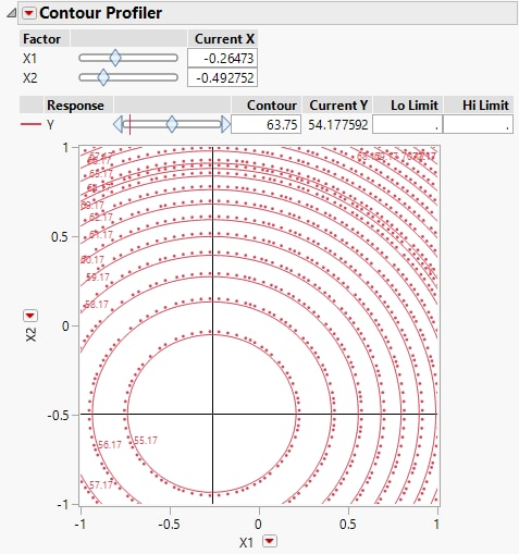
Figure 4.34 Contour Profiler with Crosshairs at Critical Point
Linking the Contour Profiler to the Prediction Profiler links the Current X values in the Contour Profiler to the X values shown in the Prediction Profiler. The X values in the Prediction Profiler give the critical point where Y is minimized. The crosshairs in the Contour Profiler show the critical point. Notice that the Current Y value is 54.177592, the predicted minimum value according to the Prediction Profiler.
Often, it is not possible to set your process factors to exactly the values that optimize the response. The Contour Profiler can help you identify alternate settings of the process factors. In the next steps, suppose that you can set your process to X1 and X2 values with only one decimal place precision, and that your process settings can vary by one decimal place in either direction of those settings.
6. In the Contour Profiler report, under Current X, type -0.3 next to X1 and -0.5 next to X2.
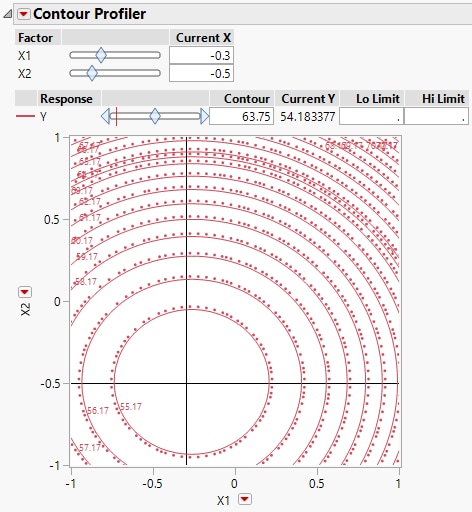
Figure 4.35 Contour Profiler Showing X1 = -0.3 and X2 = -0.5
The crosshairs are well within the innermost contour and the Current Y (the predict Y value at the Current X settings) is 54.183377, only slightly different from the predicted minimum of 54.177592.
7. In the Contour Profiler, click and drag the crosshairs to explore Current X values within a 0.1 unit radius of X1 = -0.3 and X2 = -0.5.
The predicted Y values are all below 54.4. In fact, if the settings wander to any point within the innermost contour, the predicted Y is less than the contour value of 55.17.
