Example of Constant Stress ALT Designs
Use the Constant Stress ALT Design platform to create an accelerated life test (ALT) design for one constant stress accelerating factor.
1. Select DOE > Special Purpose > Constant Stress ALT Design.
Notice that by default the design has one factor.
2. Under Factor Name, click X1 and type Temperature.
Notice that the Number of Levels value is set to 3 by default and that the Factor Transformation option is set to Arrhenius Celsius.
3. Type 10 for both the Low Usage Condition and the High Usage Condition.
Setting both the low and high usage conditions to 10 indicates that 10 is the normal usage condition.
4. Type 40 for the Low Test Condition and 80 for the High Test Condition.
5. Click Create a Plan.
Plan Specifications
Next, you set the test specifications and initial values. Use subject matter knowledge to specify the response distribution and acceleration model settings. These values are used by JMP to specify the model of interest.
1. In the Distribution Choice section, set the Response Distribution option to Weibull.
2. In the Other Specifications section, make the following selections:
– Leave the Optimality Criterion option as Quantile.
– Leave the Probability of Interest option set to 0.1 to indicate you are interested in estimating the time until 10% of units fail.
– Set the Number of Units Under Test option to 200.
– Set Length of Test option to 720 (hours) for a 30-day test.
From prior experiments, you expect 90% of units to fail by 720 hours at the high test condition.
3. In the Acceleration Models Settings section, set the Probability option to 0.9 for the high condition where temperature is 80C.
4. Leave the Weibull beta option set to 1.
5. Click Make Test Plans.
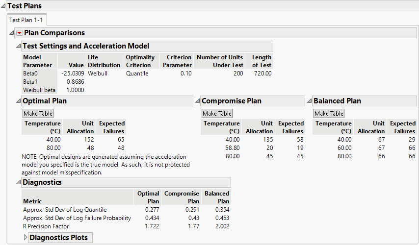
There are three test plans presented: an optimal, a compromise, and a balanced plan. The optimal design allocates 152 units to the low temperature and 48 units to the high temperature. The compromise and balanced plans allocate units across three temperature settings.
Note: The compromise plan allocates units to a temperature setting of 58.80. In practice, you would select a temperature as close to that value as possible within the precision of your temperature chamber.
Figure 22.2 Test Plans and Diagnostics
Use the diagnostics to compare the plans. For this acceleration model, all three plans have similar metrics. Select the balanced plan if you are able to run three temperature settings with an even distribution of units. Otherwise, select between the compromise and optimal plan based on test logistics.
Use the diagnostic plots to explore the sensitivity of the test plans to changes in the assumptions and to compare the three plans. The distribution profiler gives the expected failure probability as a function of temperature and time for each of the plans. Explore how the failure probability changes for each plan across the time and temperature ranges. As observed in the diagnostics, the profilers also demonstrate that there is little difference between plan types. The size of the intervals around the estimates gives a sense of the anticipated level of uncertainty for your test plan.
The R Precision Factor profiler gives the value of the metric for the temperature factor and quantile over a range of sample sizes. This gives you a sense of the anticipated uncertainty from the life test in relation to the number of samples under test. If you were able to increase your number of test units from 200 to 400, you could decrease the R precision factor. Ideally you would like the R precision to be less than one.
To save your constant stress ALT test plans, use File > Save As to save as a *.jmpdoe file.
