Example of Two-Way Analysis of Variance with an Interaction
Use the Standard Least Squares personality of the Fit Model platform to fit a two-way analysis of variance model with an interaction term. You are interested in whether the type of popcorn and the size of the batch have an effect on the yield of popcorn.
1. Select Help > Sample Data Folder and open Popcorn.jmp.
2. Select Analyze > Fit Model.
3. Select yield and click Y.
4. Select popcorn and batch and click Macros > Full Factorial.
5. Click Run.
6. Click the Response yield red triangle and select Factor Profiling > Profiler.
Report sections are shown and described below.
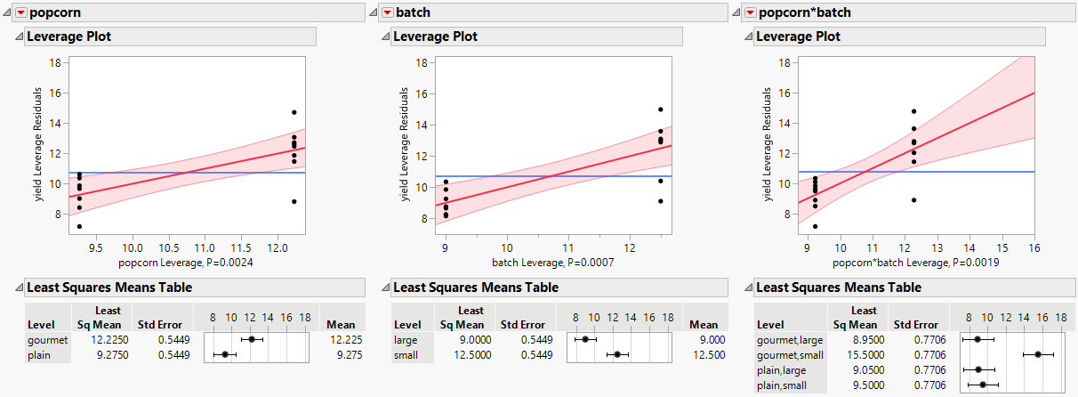
Leverage Plots
Use the leverage plots to identify influential observations and assess their impact on the regression model.
Figure 4.12 Leverage Plot and Least Squares Means Table for Factors and Their Interaction
You observe that there is a strong interaction effect between the type of popcorn and the size of the batch as indicated by the slope of the line in the leverage plot for the interaction effect.
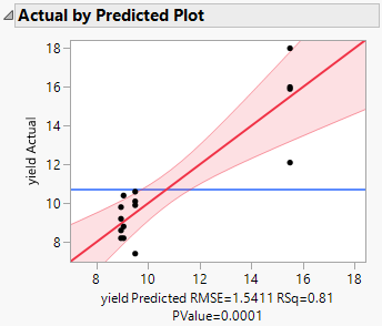
Actual by Predicted Plot
Use the Actual by Predicted Plot to assess the performance and accuracy of the model by comparing the actual values of the yield response with the predicted values from the model.
Figure 4.13 Actual by Predicted Plot
Observe that the relationship between the actual and predicted values is statistically significant (with a p-value = 0.0001).
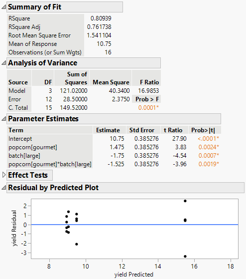
Model Fit Summary Tables and Residual Plot
Use the tables in the report to assess model fit and response variable statistics. The Summary of Fit table contains information to assess model fit and response variable statistics. The Analysis of Variance table contains information about the overall model significance and sources of variation. The Parameter Estimates table contains coefficients, standard errors, and predictor significance. The Effect Tests table contains information about the significance of individual predictors. The Residual by Predicted Plot is to evaluate the assumptions and performance of the regression model by examining the patterns or trends in the residuals across the range of predicted values.
Figure 4.14 Model Summary with ANOVA, Parameters, and Residuals
Observe that the regression model has an R-square statistic of 0.809 and a p-value of 0.0001, which both support the value of the model. Both factors and their interaction have significant effects as measured by the p-values for the test that the coefficients are zero.
The Residual by Predicted Plot shows that the residuals are randomly scattered and evenly distributed above and below the zero line. This suggests that the model assumptions are met and the residuals are normally distributed.
Effects Summary
Use the Effect Summary table to quickly assess the strength of association and statistical significance of each factor in relation to the response variable.
Figure 4.15 Effect Summary Table
All three factors exhibit high Logworth values and very small p-values, which indicates their significant impact on the response variable.
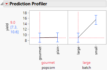
Prediction Profiler
Use the Prediction Profiler to explore how the predicted value of the response varies based on the factor settings.
Figure 4.16 Prediction Profiler


