Statistical Details for Capability Indices for Normal Distributions
This section provides details about the calculation of capability indices for normal data in the Process Capability platform.
For a process characteristic with mean μ and standard deviation σ, the population-based capability indices are defined as follows. For sample observations, the parameters are replaced by their estimates:
Cp = 
Cpl = 
Cpu = 
Cpk = 
Cpm = 
Target Index = 
The formulas use the following notation:
LSL = Lower specification limit
USL = Upper specification limit
T = Target value
For estimates of Within Sigma capability, σ is estimated using the subgrouping method that you specified. For estimates of Overall Sigma capability, σ is estimated using the sample standard deviation. If either of the specification limits is missing, the capability indices containing the missing specification limit are reported as missing.
Note: With the default AIAG (Ppk) Labeling, the indices based on Overall Sigma are denoted by Pp, Ppl, Ppu, and Ppk. The labeling for the index Cpm does not change when Overall Sigma is used. The formulas in this section are defined using Cp labels.
Confidence Intervals for Capability Indices
Confidence intervals for capability indices are available only for processes with normal distributions. Confidence intervals are calculated for both Within and Overall Sigma capability and are shown in the Individual Detail Reports.
Cp
The 100(1 - α)% confidence interval for Cp is calculated as follows:

where
 is the estimated value for Cp
 is the (α/2)th quantile of a chi-square distribution with df degrees of freedom
df is the degrees of freedom
N is the number of observations
m is the number of subgroups
For Overall Sigma capability, the degrees of freedom is equal to N - 1.
For Within Sigma capability, the degrees of freedom depends on the subgrouping and the within sigma estimation method.
• For Within Sigma capability with unbalanced subgroups, the degrees of freedom calculation is the same regardless of the within sigma estimation method. The degrees of freedom is equal to N - m.
• For Within Sigma capability with balanced subgroups of size n = N/m, the degrees of freedom calculation depends on the within sigma estimation method.
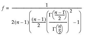
– When Within Sigma is estimated by the average of the unbiased standard deviations, the degrees of freedom is equal to f * (N - m). The scale factor f, which varies between 0.875 and 1, is defined as follows:

where Γ(n) is the gamma function evaluated at n.
For more information, see Bissell (1990).
– When Within Sigma is estimated by the average of ranges, the degrees of freedom is calculated as df = 1/A - (3/16) * A + (3/64) * A2 + 0.25. A is defined as follows:

d2(n) is the expected value of the range of n independent normally distributed variables with unit standard deviation
d3(n) is the standard deviation of the range of n independent normally distributed variables with unit standard deviation
For more information, see David (1951).
– When Within Sigma is estimated by the unbiased pooled standard deviations, the degrees of freedom is equal to N - m.
• For Within Sigma capability with no subgroups, the degrees of freedom calculation depends on the within sigma estimation method.
– When Within Sigma is estimated by the average moving ranges, the degrees of freedom is calculated as 0.62 * (N - 1).
– When Within Sigma is estimated by the median moving ranges, the degrees of freedom is calculated as 0.32 * (N - 1).
For more information, see Wheeler (2004, p. 82).
Cpk
The 100(1 - α)% confidence interval for Cpk is calculated as follows:

where
 is the estimated value for Cpk
 is the (1 - α/2)th quantile of a standard normal distribution
df is the degrees of freedom
N is the number of observations
m is the number of subgroups
For Overall Sigma capability, the degrees of freedom is equal to N - 1.
For Within Sigma capability, the degrees of freedom depends on the subgrouping and the within sigma estimation method.
• For Within Sigma capability with unbalanced subgroups, the degrees of freedom calculation is the same regardless of the within sigma estimation method. The degrees of freedom is equal to N - m.
• For Within Sigma capability with balanced subgroups of size n = N/m, the degrees of freedom calculation depends on the within sigma estimation method.
– When Within Sigma is estimated by the average of the unbiased standard deviations, the degrees of freedom is equal to f * (N - m). The scale factor f, which varies between 0.875 and 1, is defined as follows:

where Γ(n) is the gamma function evaluated at n.
For more information, see Bissell (1990).
– When Within Sigma is estimated by the average of ranges, the degrees of freedom is calculated as df = 1/A - (3/16) * A + (3/64) * A2 + 0.25. A is defined as follows:

d2(n) is the expected value of the range of n independent normally distributed variables with unit standard deviation
d3(n) is the standard deviation of the range of n independent normally distributed variables with unit standard deviation
For more information, see David (1951).
– When Within Sigma is estimated by the unbiased pooled standard deviations, the degrees of freedom is equal to N - m.
• For Within Sigma capability with no subgroups, the degrees of freedom calculation depends on the within sigma estimation method.
– When Within Sigma is estimated by the average moving ranges, the degrees of freedom is calculated as 0.62 * (N - 1).
– When Within Sigma is estimated by the median moving ranges, the degrees of freedom is calculated as 0.32 * (N - 1).
For more information, see Wheeler (2004, p. 82).
Cpm
Note: The confidence interval for Cpm is computed only when the target value is centered between the lower and upper specification limits.
The 100(1 - α)% confidence interval for Cpm is calculated as follows:

where
 is the estimated value for Cpm
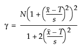
 is the (α/2)th quantile of a chi-square distribution with γ degrees of freedom

N is the number of observations
 is the mean of the observations
T is the target value
s is the sigma estimate
For Overall Sigma capability, s is the Overall Sigma estimate. For Within Sigma capability, s is replaced by the Within Sigma estimate.
Tip: For more information about confidence intervals for Cp, Cpk, and Cpm, see Pearn and Kotz (2006).
Cpl and Cpu
Lower and upper confidence limits for Cpl and Cpu are computed using the method of Chou et al. (1990).
The 100(1 - α)% confidence limits for Cpl (denoted by CPLL and CPLU) satisfy the following equations:
 where
where 
 where
where 
where
tn-1(δ) has a non-central t-distribution with n - 1 degrees of freedom and noncentrality parameter δ
 is the estimated value for Cpl
The 100(1 - α)% confidence limits for Cpu (denoted by CPUL and CPUU) satisfy the following equations:
 where
where 
 where
where 
where
tn-1(δ) has a non-central t-distribution with n - 1 degrees of freedom and noncentrality parameter δ
 is the estimated value for Cpu