Statistical Details for Custom Loss Functions
The Nonlinear platform can minimize or maximize functions other than the default sum of squares residual. This section shows the mathematics of how it is done.
Suppose that f(β) is the model. Then the Nonlinear platform attempts to minimize the sum of the loss functions defined as follows:

The loss function ρ(•) for each row can be a function of other variables in the data table. It must have nonzero first- and second-order derivatives. The default ρ(•) function, squared-residuals, is

To specify a model with a custom loss function, construct a variable in the data table and build the loss function. After launching the Nonlinear platform, select the column containing the loss function as the loss variable.
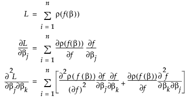
The nonlinear minimization formula works by taking the first two derivatives of ρ(•) with respect to the model, and forming the gradient and an approximate Hessian as follows:

If f(•) is linear in the parameters, the second term in the last equation is zero. If not, you can still hope that its sum is small relative to the first term, and use

The second term is probably small if ρ is the squared residual because the sum of residuals is small. The term is zero if there is an intercept term. For least squares, this is the term that distinguishes Gauss-Newton from Newton-Raphson.
Note: The standard errors, confidence intervals, and hypothesis tests are correct only if least squares estimation is done, or if maximum likelihood estimation is used with a proper negative log-likelihood.