Specify a By Variable
In many JMP platforms, you can specify columns as By variables. To do this in a script, include a By argument in the platform command, listing each column as an argument.
The following example uses the Big Class.jmp data table, which contains the names, ages, sex, heights, and weights for 40 students. Create a bivariate report of weight by height, using sex as a By variable, and adding a variety of fits.
Create the Bivariate Report Using a By Variable
1. Select File > New > Script.
2. Add the following lines:
dt = Open( "$SAMPLE_DATA/Big Class.jmp" );
biv = dt << Bivariate( Y( weight ), X( height ), By( sex ));
The first line opens the Big Class.jmp sample data table. The second line creates a platform object called biv that runs a bivariate report of weight and height by sex.
3. Click Run Script  .
.
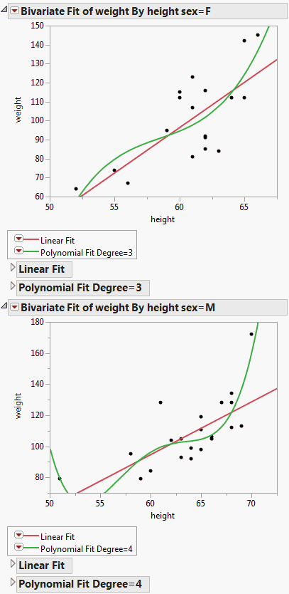
The report window shows two graphs, one where sex is F and one where sex is M.
Send Messages to the Entire Platform or to a Single By Level
1. If you do not have the log showing, turn it on. Right-click in the script and select Show Embedded Log.
2. Add this line to the script:
Show( biv );
3. Highlight the Show( biv ) line and click Run Script  .
.
In the log, rather than returning a single reference to a platform, Bivariate[], the platform object returns a list of references: biv = {Bivariate[], Bivariate[]}. The two references correspond to the two levels (F and M) of the By variable, sex.
You can direct messages to each By level individually or to all By levels.
4. Send a message to all By levels to add a linear regression fit. Add this line to the script:
biv << Fit Line;
5. Highlight the line you just created and click Run Script  .
.
In the report window, a linear regression line is added to both graphs, with the corresponding Linear Fit reports.
6. Send a message to only the F level, adding a cubic polynomial fit. Add this line to the script:
biv[1] << Fit Polynomial( 3 );
Tip: The number for each By level corresponds to their order in the report window, which is usually alphanumeric. If the By column contains a Value Order column property, that ordering is followed.
7. Highlight the line you just created and click Run Script  .
.
In the report window, a polynomial fit line is added to the F graph, with the corresponding Polynomial Fit reports.
8. Send a message only to the M level, adding a quartic polynomial fit. Add this line to the script:
biv[2] << Fit Polynomial( 4 );
9. Highlight the line you just created and click Run Script  .
.
In the report window, a quartic fit line is added to the M graph, with the corresponding Polynomial Fit reports.
Figure 10.2 By Group Reports
If you specify more than one column in By argument, graphs appear for each subgroup of each By variable. In this example, By( sex, age ) would produce graphs for females age 12, females age 13, and so on, up to age 17. It would also produce graphs for males age 12 up to age 17.
Extract Results from a Report
The following example shows how to launch a platform with By groups and extract results (in this case, variances) from each group:
dt = Open( "$SAMPLE_DATA/Big Class.jmp" );
// onew is the JSL variable holding a list of platforms
onew = dt << Oneway( x( :age ), y( :height ), by( :sex ), anova );// r is a list of reports
r = onew << Report;// nBy is the number of reports generated
nBy = N Items( r );// vc is an array of as many rows as reports, one column, all set to zero
vc = J( nBy, 1, 0 );
// for each report, do the following:
For( i = 1, i <= nBy, i++,
vc[i] = r[i] // vc[i] is the variance of the ith report[Outline Box( "Analysis of Variance" ), // look for this outline
// then look for this column and get the second value
Column Box( "Sum of Squares" )][2]
);
Show( vc ); // debugging, look in log to see this value
// byValues becomes a list of the values in the sex column
Summarize( byValues = By( :sex ) );// make a new table with two rows (M.F) and two columns
New Table( "Variances" )
<< New Column( "Sex", // create a new column called Sex
character,
width( 8 ),values( byValues )
// create a new column called Variance
) << New Column( "Variance", Numeric, "Continuous", Values( vc ) );
