Statistical Examples

This section contains statistical examples of using matrices.

Suppose that you want to implement your own regression calculation, rather than use the facilities built into JMP. Because of the compact matrix notation, it might require only a few lines of code:

Y = [98, 112.5, 84, 102.5, 102.5, 50.5, 90, 77, 112, 150, 128, 133, 85, 112];

X = [65.3, 69, 56.5, 62.8, 63.5, 51.3, 64.3, 56.3, 66.5, 72, 64.8, 67, 57.5, 66.5];

X = J( N Row( X ), 1 ) || X; // put in an intercept column of 1s

beta = Inv( X` * X ) * X` * Y; // the least square estimates

resid = Y - X * beta; // the residuals, Y - predicted

sse = resid` * resid; // sum of squared errors

Show( beta, sse );

This could be expanded into a script that gets its data from a data table, calculates additional results, and shows the results in a report window:

// open the data table

dt = Open( "$SAMPLE_DATA/Big Class.jmp" );

// get data into matrices

x = (Column( "Age" ) << Get Values ) || (Column( "Height" ) << Get Values);

x = J(N Row( x ), 1, 1) || x;

y = Column( "Weight" ) << Get Values;

// regression calculations

xpxi = Inv( x` * x );

beta = xpxi * x` * y; // parameter estimates

resid = y - x * beta; // residuals

sse = resid` * resid; // sum of squared errors

dfe = N Row( x ) - N Col( x ); // degrees of freedom

mse = sse / dfe; // mean square error, error variance estimate

// additional calculations on estimates

stdb = Sqrt( Vec Diag( xpxi ) * mse ); // standard errors of estimates

alpha = .05;

qt = Students t Quantile( 1 - alpha / 2, dfe );

betau95 = beta + qt * stdb; // upper 95% confidence limits

betal95 = beta - qt * stdb; // lower 95% confidence limits

tratio = beta :/ stdb; // Student's T ratios

probt = ( 1 - TDistribution( Abs( tratio ), dfe ) ) * 2; // p-values

// present results

New Window( "Big Class Regression",

Table Box(

String Col Box( "Term",{"Intercept", "Age", "Height"} ),

Number Col Box( "Estimate", beta ),

Number Col Box( "Std Error", stdb ),

Number Col Box( "TRatio", tratio ),

Number Col Box( "Prob>|t|", probt ),

Number Col Box( "Lower95%", betal95 ),

Number Col Box( "Upper95%", betau95 ) ) );

ANOVA Example

You can implement your own one-way ANOVA. This example presents a problem involving a three-level factor indicating Low, Medium, and High doses and a response measurement. Therefore, this example solves the general linear model, as follows:

Y = a + bX + e

Where:

•

Y is a vector of responses

•

a is the intercept term

•

b is a vector of coefficients

•

X is a design matrix for the factor

•

e is an error term

factor = [1, 2, 3, 1, 2, 3, 1, 2, 3];

y = [1, 2, 3, 4, 3, 2, 5, 4, 3];

First, build a design matrix for the factor:

Design Nom( factor );

[1 0, 0 1, -1 -1, 1 0, 0 1, -1 -1, 1 0, 0 1, -1 -1]

Next, add a column of 1s to the design matrix for the intercept term. You can do this by concatenating J and Design Nom(), as follows:

x = J( 9, 1, 1) || Design Nom( factor );

Now, to solve the normal equation, you need to construct a matrix M with partitions:

You can construct matrix M in one step by concatenating the pieces, as follows:

M = ( x` * x || x` * y )

( y` * x || y` * y );

Now, sweep M over all the columns in X’X for the full fit model, and over the first column only for the intercept-only model:

FullFit = Sweep( M, [1, 2, 3] ); // full fit model

InterceptOnly = Sweep( M, [1] ); // model with intercept only

Recall that some of the standard ANOVA results are calculated by comparing the results of these two models. This example focuses on the full fit model, which produces this swept matrix:

[0.111111111111111 0 0 3,

0 0.222222222222222 -0.11111111111111 0.333333333333333,

0 -0.11111111111111 0.222222222222222 0,

-3 -0.33333333333333 0 11.33333333333333]

Examine the model coefficients from the upper right partition of the matrix. The lower left partition is the same, except that the signs are reversed: 3, 0.333, 0. The results can be interpreted as follows:

•

The coefficient for the intercept term is 3.

•

The coefficient for the first level of the factor is 0.333.

•

The coefficient for the second level is 0.

•

Because of the use of Design Nom(), the coefficient for the third level is the difference, –0.333.

•

The lower right partition of the matrix holds the sum of squares, 11.333.

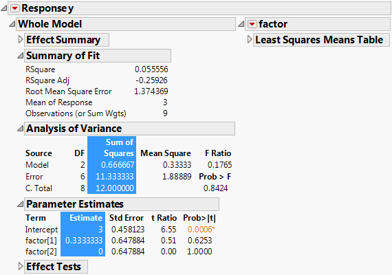
You could modify this into a generalized ANOVA script by replacing some of the explicit values in the script with arguments. These results match those from the Fit Model platform. See 图 7.1.

图 7.1 ANOVA Report Within Fit Model

Construct the report in 图 7.1 as follows:

Build a data table (described in the “Data Tables” chapter on page 303):

dt = New Table( "Data" );

dt << New Column( "y", Set Values( [1, 2, 3, 4, 3, 2, 5, 4, 3] ) );

dt << New Column( "factor", "Nominal", Values( [1, 2, 3, 1, 2, 3, 1, 2, 3] ) );

Run a model (described in “Launch the Analysis and Save the Script to a Window” on page 438 in the “Scripting Platforms” chapter):

obj = Fit Model(

Y( :y ),

Effects( :factor ),

Personality( "Standard Least Squares" ),

Run(

y << {Plot Actual by Predicted( 0 ), Plot Residual by Predicted( 0 ),

Plot Effect Leverage( 0 )}

)

);

Use JSL techniques for navigating displays (described in “Display Box Object References” on page 486 in the “Display Trees” chapter):

ranova = obj << Report;

ranova[Outline Box( 6 )] << Close( 0 );

ranova[Outline Box( 7 )] << Close( 1 );

ranova[Outline Box( 9 )] << Close( 1 );

ranova[Outline Box( 5 ), Number Col Box( 2 )] << Select;

ranova[Outline Box( 6 ), Number Col Box( 1 )] << Select;

The result is shown in 图 7.1.