Plot Functions

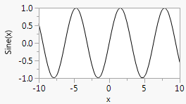
A Y Function() function is used to draw smooth functions. The first argument is the expression to be plotted. The second argument is the name of the X variable in the expression.

win = New Window( "Sine Function",

Graph Box(

Frame Size( 200, 100 ),

X Scale( -10, 10 ),

Y Scale( -1, 1 ),

X Name( "x" ),

Y Name( "Sine(x)" ),

Y Function( Sine( x ), x ) ) );

图 12.32 Sine Wave

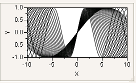
You can use For to overlap several sine waves:

win = New Window( "Overlapping Sine Waves",

Graph Box(

Frame Size( 200, 100 ),

X Scale( -10, 10 ),

Y Scale( -1, 1 ),

For( i = 1, i <= 4, i += .1,

Y Function( Sine( x / i ), x )

)

);

图 12.33 Overlapping Sine Waves

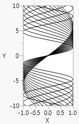
Similarly, X Function() is for drawing a graph where the symbol is varied on the Y variable.

win = New Window( "Overlapping Sine Waves",

Graph Box(

Frame Size( 100, 200 ),

X Scale( -1, 1 ),

Y Scale( -10, 10 ),

For( i = 1, i <= 4, i += .2,

X Function( Sine( y / i ), y )

)

);

图 12.34 Overlapping Sine Waves along the X-Axis

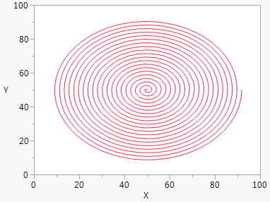
An XY Function() draws a smooth curve using a pair of formulas (parametric equations) that depend on a third variable. The third variable’s value is incremented from a minimum value to a maximum value to generate the X-Y pairs.

win = New Window( "Spiral",

Graph Box(

Pen Color( "red" ); // red line color

xCenter = 50; // location of the center of the curve on the x axis

yCenter = 50; // location of the center of the curve on the y axis

minAngle = 0;

maxAngle = Pi() * 2 * 20;

XY Function(

xCenter + ((ta / 3) * Cos( ta )),

yCenter + ((ta / 3) * Sin( ta )),

ta,

Min( minAngle ),

Max( maxAngle ),

Inc( Pi() / 100 )

);

)

);

In this example, Sin() and Cos() use ta as an argument (rotates) and as a factor (expands). (Sin() and Cos() use radians, not degrees.)

图 12.35 Spiral Parametric Plot

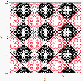
Contour Function() is an analogous way to represent a three-dimensional function in a two-dimensional space. The final argument specifies the value(s) for the contour line(s). The argument can be a value, an indexed range of values using ::, or a matrix of values.

win = New Window( "Bird's eye view of the egg carton function",

Graph Box(

Frame Size( 300, 300 ),

X Scale( -10, 10 ),

Y Scale( -10, 10 ),

Pen Color( "black" );

Pen Size( 2 );

Contour Function( Sine( y ) + Cosine( x ), x, y, (0 :: 20) / 5 );

Pen Color( "red" );

Pen Size( 1 );

Contour Function( Sine( y ) + Cosine( x ), x, y, (-20 :: 0) / 5 );

)

);

图 12.36 Egg Carton Function

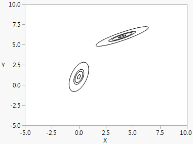
Normal Contour() draws normal probability contours for k populations and two variables. The first argument is a scalar probability or a matrix of probability values for the contours. Subsequent arguments are matrices to specify means, standard deviations, and correlations. The mean and standard deviation matrices have dimension k × 2. The correlation matrix should be k × 1, where the first row pertains to the first contour, the second row to the second contour, and so on. The first column is for x and the second column for y. Consider the following example:

The following script draws contours at probabilities 0.1, 0.5, 0.7, and 0.99 for two populations and two variables. The first population has x mean 0 and y mean 1, with standard deviation 0.3 along the x axis and 0.6 along the y-axis, and with correlation 0.5. The second has x mean 4 and y mean 6, with standard deviation 0.8 along the x axis and 0.4 along the y-axis, and with correlation 0.9.

win = New Window( "Normal Contours",

Graph Box(

X Scale( -5, 10 ),

Y Scale( -5, 10 ),

Normal Contour( [.1, .5, .7, .99], [0 1, 4 6], [.3 .6, .8 .4], [.5, .9] )

)

);

图 12.37 Normal Contour Function

Normal Contour() is a general way to accomplish effects such as Bivariate’s density ellipses. The Bivariate script in the Football.jmp sample data creates an example.

Gradient Function

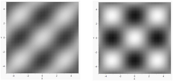
Gradient Function() fills a set of rectangles on a grid according to a color determined by the expression value as it crosses a range corresponding to a range of colors.

Gradient Function( expression, xname, yname, [zlow, zhigh], ZColor( [colorLow, colorHigh] ), <XGrid( min, max, incr )>, <YGrid( min, max, incr )>, <Transparency( t )>;

Here are explanations of the elements in the Gradient Function() syntax:

GradientFunction(

expression

// The expression to be contoured, which is a function in terms of the two variables that follow

xname,yname,

// The two variable names used in the expression

[zlow, zhigh],

// The low and high expression values the gradient is scaled between

ZColor([colorLow, colorHigh])

// The colors that correspond to the low value and the high value

<XGrid(min, max, incr),>

<YGrid(min, max, incr)> );

// Optional specification for the grid of values

// The value 0 means clear. The value 1 means completely opaque and is the usual drawing mode.

The ZColor() values must be numeric codes rather than names. You can use the color menu indices (such as 0=black, 1=grey, 2=white, 3=red, 4=green, and 5=blue) found in Specify Colors.

The following example uses Gradient Function() to create an animated graph.

phase = 0.7;

win = New Window( "Gradient Function",

a = Graph(

Frame Size( 400, 400 ),

X Scale( -5, 5 ),

Y Scale( -5, 5 ),

Gradient Function(

phase * Sine( x ) * Sine( y ) + (1 - phase) * Cosine( x ) * Cosine( y ),

[-1 1],

zcolor( [0, 2] )

)