Model Results (Genomic Bayesian Regression)
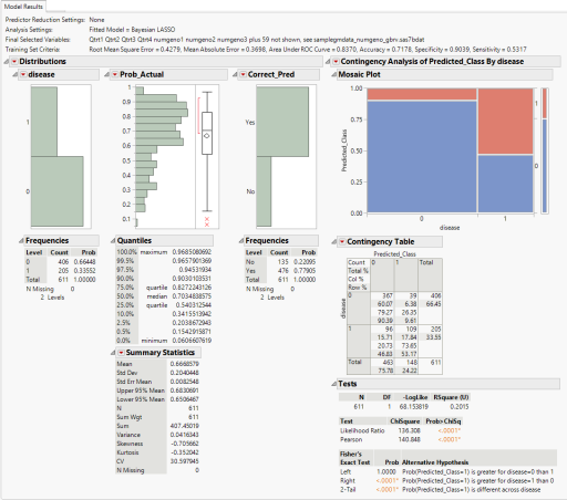
The Model Results tab is shown below:

The Model Results tab contains the following elements:
| • | Summary of Model Fit |
This top section of the tab echoes the key parameter settings for the model fit. It also lists the final selected variables and standard model fitting criteria for the training and test sets such as Root Mean Square Error, Mean Absolute Error, Area Under the ROC Curve, Accuracy, specificity (for binary dependent variables), sensitivity (for binary dependent variables), category-specific Accuracy (for non-binary categorical dependent variables), and Harrell's C-Statistic (for continuous dependent variables).
| • | Distributions |
This section first plots the distribution of the dependent variable. If it is categorical, the distribution of the posterior probability of having the true value (Prob_Actual) is plotted. Values below 0.5 for this variable indicate misclassifications. For categorical dependent variables, the distribution of the correctness of the prediction (Correct_Pred) is present. Note the fraction of "Yes" values for this variable is the same as the Accuracy statistic.
For continuous dependent variables, this section contains the distribution of the predicted values and residuals.
You should study these distributions carefully to make sure results make sense based on your knowledge of the data and model. Click on histogram bars to highlight observations of interest. To view the underlying data table, go to the Tabs section in the upper left corner and click Model Results > View Data. Press to find the first selected row.
See Distribution for more information.
| • | Contingency Analysis (for categorical dependent variables) |
This section includes a mosaic plot and contingency table of the prediction confusion matrix. It breaks down all correct and incorrect predictions into cells.
You can see which categories are predicted poorly and view patterns of misclassification. As with histogram bars, click on mosaic cells to highlight observations of interest. To view the details in the underlying data table, go to the Tabs section in the upper left corner and click Model Results > View Data.
See Contingency Table and Contingency Table for more information.
| • | Bivariate Fits (for continuous dependent variables) |
This section includes bivariate plots of both actual value and residuals versus predicted values. The latter is actually a 45-degree clockwise rotation of the former. These plots can help identify the quality of model fit and outliers in the data. The ideal residual plot is random noise around a zero horizontal line; the estimated smoothing spline should be close to horizontal in this case. Deviations from this can be a sign of a poor model, missing predictors, or a dependent variable that is very difficult to predict.