Process Description

Population Measures

The Population Measures process creates a symmetric matrix of dissimilarities between specified groups within a study. Genetic distance computation is based on differences in group allele frequencies calculated using PROC ALLELE for each marker variable. Groups are determined by the input values of the specified population variable. Multiple genetic distance matrices can be output for separate sets of marker variables if an annotation By Group variable is specified.

This process also produces Wright's F statistics (Wright, 1951) measuring the degree of relatedness between different types of allele pairs. Cockerham (1969, 1973) defines these same quantities in an analysis of variance (ANOVA) framework. For a population hierarchy defined by the Population Variable, the measures computed as Pop Theta, Within Pop f, and Overall F correspond to Wright's F_ST, and, when HWE is not assumed, F_IS and F_IT. A weighted average of these measures over all loci is also reported as an overall estimate as well as measures for individual loci are reported. The estimates of these parameters are calculated using an ANOVA structure along with a method-of-moments approach.

Matrices produced by this process can be used as input for the Multidimensional Scaling process.

Refer to the SAS/Genetics User's Guide for more information.

What do I need?

One data set is required to run the Population Measures process. This Input Data Set, contains all of the marker data.

The hapmap_subset.sas7bdat data set used in the following example was generated from data downloaded from the HapMap project (http://hapmap.ncbi.nlm.nih.gov/), as follows. Unzipped .txt files containing SNP data from chromosome 21, NCBI Build 35, of individuals from four different populations (Utah residents with ancestry from northern and western Europe (CEU), Han Chinese residents of Beijing (HCB), Japanese residents of Tokyo (JPT), and members of the Yoruba group in Ibadan, Nigeria (YRI)) were imported. The resulting SAS data sets were appended and then filtered to remove related individuals using pedigree information provided by the HapMap project (ftp://ftp.ncbi.nlm.nih.gov/hapmap/samples_individuals/). The resulting data set was subjected to both the Marker Properties and Subset and Reorder Genetic Data processes to eliminate low quality (as defined by low MAFs and low Call Rates) SNPs. Finally, 500 markers were selected at random to generate the hapmap_subset.sas7bdat data set. This data set consists of 208 rows of individuals with 500 columns corresponding to SNP marker data on these individuals. Marker data is presented in the one-column genotypic format with delimited alleles. This data set is partially shown below.

Note: The hapmap_subset.sas7bdat data set is a wide data set; markers are listed in columns, whereas individuals are listed in rows.

A second, optional, data set that can be used in this process is the Annotation Data Set. This data set contains information, such as gene identity or chromosomal location, for each of the markers.

The hapmap_subset.sas7bdat data set is located in the Sample Data folder.

For detailed information about the files and data sets used or created by JMP Genomics software, see Files and Data Sets.

Output/Results

The output of this process includes three output data sets, two plots, and a set of AceView Database. The data sets and plots are accessed from a tabbed Results window.

This process was run for the data sets shown above.

A Heat Map and Dendrogram showing the hierarchical clustering of the genetic distances calculated in this process is shown below.

Populations with smaller genetic distance measures are more genetically similar. In this example, JPT and CHB (Japanese and Chinese populations) are very close as measured by Reynolds' distance. Conversely, the Yoruban population is more genetically distinct from JPT and CHB.

The hapmap_subset_pmd.sas7bdat matrix (shown below), used to generate this heat map, is suitable for further analyses. Use the action button to load the output matrix directly into the Multidimensional Scaling process.

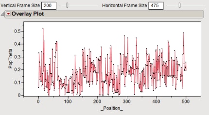
Finally, two output data sets (not shown), listing individual and overall F-statistics, are generated. The results across the region spanned by the markers, are displayed in the Overlay Plot shown below.