where Fi(x) is one of the supported distributions, k is the number of components in the mixture, and the wi are positive weights that sum to 1. The Fit Mixture option attempts to identify clusters of observations that are drawn from each of the component distributions, Fi(x). It estimates the parameters of the mixture and the probability that an observation is drawn from any given component.
The fitting methodology is based on assumptions about the underlying clusters, called the Starting Value Method. Suppose that you designate k distributions. There are three Starting Value Methods:
|
•
|
Separable Clusters assumes that the ingredient distributions affect some observations more profoundly than others. For separable clusters, each of the k densities has an identifiable mode and defines a cluster.
|
|
•
|
Overlapping Clusters assumes a situation that is intermediate between Single Cluster and Separable Clusters. Some densities stand out, but others jointly affect a portion of the observations. In this case, there are m clusters in the data, where m is less than k, the total number of densities.
|
Select the number of components in the mixture distribution that have the given distribution. The sum of the Quantity values is k, the number of densities in the mixture.
Select a method that reflects your assumptions about the mixture. See Model Fit and Mixture Starting Value Methods.
Click Go to fit the desired mixture. The Model List is updated with the model that you fit, and a report with the name of the mixture model is added.
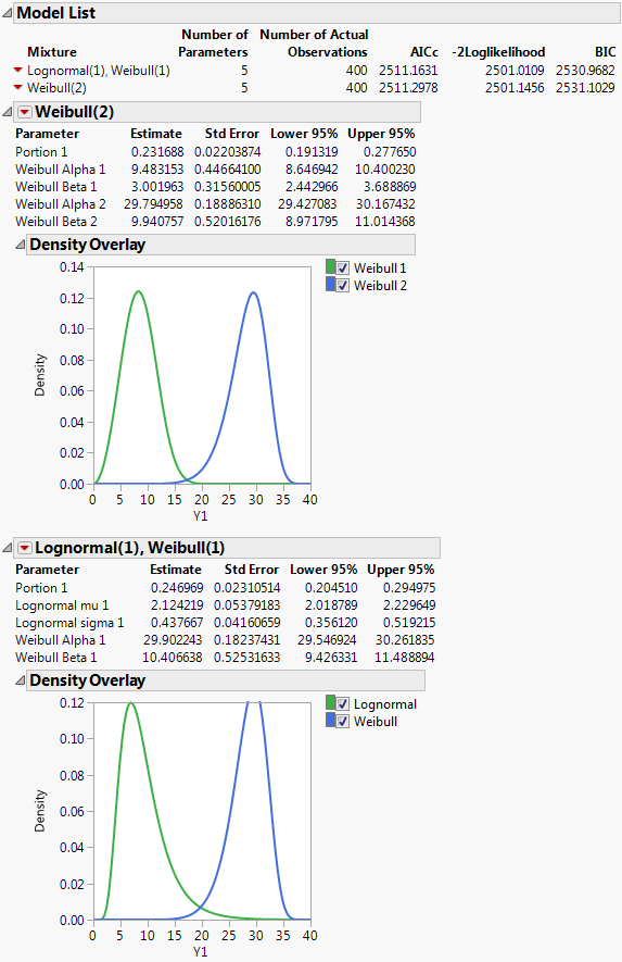
The Model List report lists the mixture distributions that you fit. The report provides the number of parameters, the number of actual observations, and the AICc, -2*LogLikelihood, and BIC statistics for each mixture distribution. For more details about these statistics, see Likelihood, AICc, and BIC in the Fitting Linear Models book.
|
•
|
The Comparison Criterion red triangle option does not affect the order of models in the Model List.
|
|
•
|
Parameter estimates are given for each distribution in the mixture. The Parameter column also includes parameters called Portion <i>, where i = 1, 2, .., k-1. These are estimates of the weights wi for the mixture. Since the weights sum to 1, the kth weight can be computed from the first k - 1 weights.
Shows four types of profilers for the combined mixture distribution F. See Mixture Profiler Options for a description of their red triangle options.
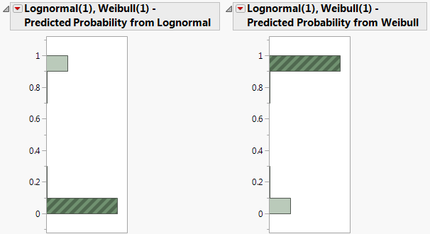
For each mixture density, saves a column to the data table containing the probability that an observation belongs to that density. For the formulas used in the calculation, see Fit Mixture Save Predictions Formulas.
Displays a window for each factor allowing you to enter a specific value for the factor’s current setting, to lock that setting, and to control aspects of the grid. For details, see Reset Factor Grid in the Profilers book.
Provides a menu that consists of options relating to profiler settings, scripts, and linking profilers. For details, see Factor Settings in the Profilers book.
|
1.
|
|
2.
|
Select Analyze > Reliability and Survival > Life Distribution.
|
|
3.
|
|
4.
|
Click OK.
|
|
5.
|
Select Fit Mixture from the red triangle menu next to Life Distribution.
|
|
6.
|
|
7.
|
Select Separable Clusters in the Starting Value Methods panel.
|
|
8.
|
Click Go.
|
Figure 2.10 Fit Mixture for Weibull (2)
|
9.
|
|
10.
|
Click Go.
|
Figure 2.11 Fit Mixture for Lognormal(1), Weibull(1)
|
1.
|
From the Lognormal(1), Weibull(1) red triangle menu, select Save Predictions.
|
|
2.
|
Select Analyze > Distribution.
|
|
4.
|
Check Histograms Only.
|
|
5.
|
Click OK.
|
|
6.
|
In the histogram for Lognormal(1), Weibull(1) - Predicted Probability from Weibull, click in the bar corresponding to the value near 1.
|
Figure 2.12 Histograms for Mixture Probabilities


