Simple Linear Path

To model linear degradation paths, select Degradation Path Style > Simple Linear Path from the Degradation Data Analysis red triangle menu.

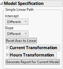
Use the Simple Linear Path Model specification to specify the form of the linear model that you want to fit to the degradation path. You can model linear paths, or nonlinear paths that can be transformed to linear.

Figure 7.5 Simple Linear Path Model Specification 

The Simple Linear Path model specification contains the following options:

Intercept

Specifies the form of the intercept in the model:

Different

Fits a different intercept for each level of the ID variable.

Common in Group

Fits the same intercept for each level of the ID variable in the same level of the X variable, and fits different intercepts between levels.

Common

Fits the same intercept for all levels of the ID variable.

Zero

Restricts the intercept to be zero for all levels of the ID variable.

Slope

Specifies the form of the slope in the model:

Different

Fits a different slope for each level of the ID variable.

Common in Group

Fits the same slope for each level of the ID variable in the same level of the X variable, and fits different slopes between levels.

Common

Fits the same slope for all levels of the ID variable.

Reset Axes to Linear

Resets the Overlay plot axes to their initial settings.

<Y, Response> Transformation

If a transformation on the Y variable can linearize the degradation path, select the transformation (Linear, ln(x), exp(x), x^2, sqrt(x) or Custom) here. For more information about the Custom option, see Custom Transformations.

<Time> Transformation

If a transformation for the Time variable can linearize the degradation path, select the transformation (Linear, ln(x), x^2, sqrt(x) or Custom) here. For more information about the Custom option, see Custom Transformations.

Generate Report for Current Model

Creates a report for the current model settings. This includes a Model Summary report, and Estimates report giving the parameter estimates. See Degradation Model Summary Reports.

Custom Transformations

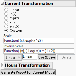
If you need to perform a transformation that is not given, use the Custom option. For example, to transform the response variable using exp(-x2), enter the transformation as shown in the Scale box in Figure 7.6. Also, enter the inverse transformation in the Inverse Scale box.

Note: JMP automatically attempts to solve for the inverse transformation. If it can solve for the inverse, it automatically enters it in the Inverse Scale box. If it cannot solve for the inverse, you must enter it manually.

Figure 7.6 Custom Transformation Options 

Name the transformation using the text box. When finished, click the Use & Save button to apply the transformation. Select a transformation from the menu if you have created multiple custom transformations. Click the Delete button to delete a custom transformation.