 Additional Example of Multivariate Embedding
In this example, you use the same data set as in Example of Multivariate Embedding, but reduce the data to three dimensions instead of two. You also compare the results between the UMAP method and the t-SNE method.
1. Select Help > Sample Data Folder and open Cytometry.jmp.
2. Select Analyze > Multivariate Methods > Multivariate Embedding.
3. Select CD3 through MCB and click Y, Columns.
4. Assign t-SNE as the Method.
5. Type 3 next to Output Dimensions.
6. (Optional.) Type 1234 next to Random Seed.
Note: Entering the seed above enable you to reproduce the results shown in this example.
7. Select Keep dialog open.
8. Click OK.
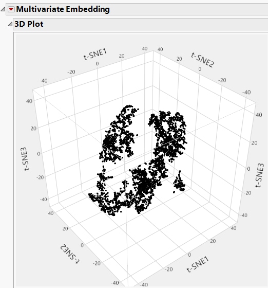
Figure 11.4 Example of a 3D t-SNE Plot
9. In the launch window, change Method to UMAP.
10. Click OK.
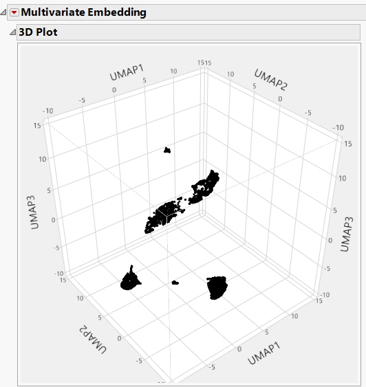
Figure 11.5 Example of a 3D UMAP Plot
Each 3D plot shows the coordinates for the first three embedded components of the corresponding dimensional reduction method. Comparing the UMAP and t-SNE method, the UMAP method took less computation time while also providing tighter clustering of the data. There are more distinct clusters visible in the 3D UMAP plot as compared to the 3D t-SNE plot in Figure 11.4.
Tip: You can rotate the grid to view the clusters more clearly.

