 Example of a Uniformity Trial
Use the Mixed Model personality of the Fit Model platform to analyze a uniformity trial. You are interested in analyzing an agronomic uniformity trial that was conducted on an 8x8 grid of plots. In a uniformity trial, a test crop is grown on a field with no experimental treatments applied. The response variable, often yield, is measured. The idea is to characterize variability in the field as background for planning a designed experiment to be conducted on that field.
Your objective is to use the information from these data to design a yield trial with 16 treatments. Specifically, you want to decide whether to conduct future experiments on the field:
• a complete block design with 4 blocks (denoted Quarter in the data)
• an incomplete block design with 16 blocks (denoted Subquarter in the data)
• a completely randomized design with spatially correlated errors
With this objective, spatial data can be treated as repeated measures with two or more dimensions as repeated effects. So, you can compare and choose an appropriate model using the values in the Fit Statistics report. You start by determining if there is significant spatial variability, then you determine whether there is a nugget effect.
Once you have established whether there is a nugget effect, you determine the best fitting spatial covariance structure. Finally, you fit the blocking models and compare these to the best spatial structure. In this example, both AICc and BIC are used to select a best model. Spatial Correlation Structure provides more information about nugget effects and other spatial terminology.
Tip: This section walks you through many aspects of fitting spatial data (from fitting the model to deciding on the best covariance structure). Leave the Fit Model launch window open as you work through each example.
 Fit a Spatial Structure Model
To determine whether there is significant spatial variability, you can fit a model that accounts for spatial variability. Then you can compare the likelihood for this spatial model to the likelihood for a model that does not account for spatial variability. You can do this because the independent errors model is nested within the spatial model family: The independent errors model is a spatial model with spatial correlation, ρ, equal to 0. This means that you can perform a formal likelihood ratio test of the two models.
First, fit the model that accounts for spatial structure.
1. Select Help > Sample Data Folder and open Uniformity Trial.jmp.
2. Select Analyze > Fit Model.
3. Select Keep dialog open so that you can return to the launch window in the next example.
4. Select Yield and click Y.
5. Select Mixed Model from the Personality list.
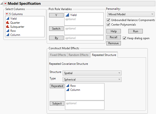
6. Select the Repeated Structure tab.
7. Choose Spatial from the list next to Structure.
8. Choose Spherical from the list next to Type.
9. Select Row and Column and click Repeated.
Figure 8.32 Completed Fit Model Launch Window Showing Repeated Structure Tab
10. Click Run.
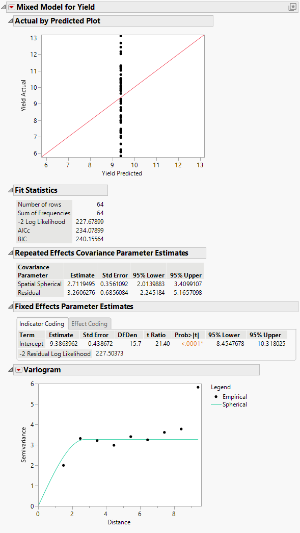
Figure 8.33 Mixed Model Report for Spatial Spherical Covariance Structure
In the Mixed Model report, the Actual by Predicted Plot shows that the predicted yield is a single value. This is because only spatial covariance was fit. The Fit Statistics report shows that -2 Log Likelihood is 227.68, and the AICc is 234.08.
Because an isotropic spatial structure was fit, a Variogram plot is shown. Because the trials are laid out in an 8 by 8 grid, there are more pairs of points at small distances than at very large distances. See Figure 8.37 for the layout. The Variogram shows that a spherical spatial structure is an excellent fit for distances up to about 8.4. The distance class for the final distance consists of only the two diagonal pairs of points.
The Repeated Effects Covariance Parameter Estimates report gives estimates of the range (Spatial Spherical = 2.71) and the sill (Residual = 3.26). See Variogram.
 Fit the Independent Errors Model
Next, fit the independent errors model.
1. Return to the Fit Model Launch Window.
2. Select Repeated Structure tab.
3. Select Residual from the Structure list.
4. Remove Row and Column from the Repeated effects list.
Otherwise, a warning appears: “Repeated columns and subject columns are ignored when the Residual covariance structure is selected.”
5. Click Run.
The fit statistics for the independent errors model are: -2 Log Likelihood = 254.22, and AICc = 258.41. Each of these exceeds the corresponding value for the spatial correlation model, where -2 Log Likelihood is 227.68 and the AICc is 234.08. Because smaller values of these statistics indicate a better fit, the spatial model might provide a better fit.
 Conduct a Likelihood Ratio Test (Optional)
A formal likelihood ratio test shows whether the spatial correlation model explains significant variation. One model must be nested in another model to create valid likelihood ratio tests.
Typically, spatial models are compared using AICc or BIC rather than through formal likelihood ratio testing. Evaluating the AICc or BIC is faster, and many spatial models are not nested.
You can conduct a likelihood ratio test in this example, because the independent errors model is nested within the spatial model family. The independent errors model is a spatial model with spatial correlation, ρ, equal to 0. This means that you can perform a formal likelihood ratio test of the two models.
In this example, the likelihood ratio test statistic is 254.22-227.68=26.54. Comparing this to a Chi-square distribution on one degree of freedom, the null hypothesis of no spatial correlation is rejected with a p-value < 0.0001. You can conclude that these data contain significant spatial variability.
 Select the Type of Spatial Covariance
Next, you determine which spatial covariance structure best fits the data:
• with or without a nugget effect (variation over relatively small distances)
• isotropic (spatial correlation is equal in all directions) or anisotropic (spatial correlation differs in the two directions)
• type of structure, spherical, Gaussian, exponential, or power.
1. Return to the Fit Model launch window.
2. Select the Repeated Structure tab.
3. Select Row and Column and click Repeated.
4. Select Spatial with Nugget from the Structure list.
5. Select Spherical from the Type list.
6. Click Run.
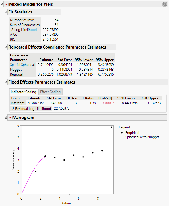
The Mixed Model report is shown in Figure 8.34. Notice that the log-likelihoods are essentially equal to those of the spherical with no nugget model, and the AICc is slightly higher (236.36 compared to 234.08). The Repeated Effects Covariance Parameter Estimates report shows that the Nugget covariance parameter has an estimate of zero. There does not appear to be any evidence for a nugget effect.
Figure 8.34 Mixed Model Report for Spatial Spherical with Nugget
7. Click the Variogram red triangle and select Spatial > Spherical.
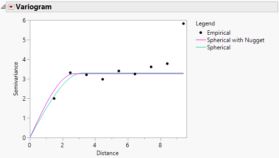
Figure 8.35 Variogram in the Mixed Model Report
The two variograms are virtually identical. This also suggests that there is no evidence of a nugget effect.
8. Return to the Fit Model launch window.
9. Select Repeated Structure tab.
10. To test anisotropicity, select Spatial Anisotropic from the Structure list.
11. Select Spherical from the Type list.
12. Click Run.
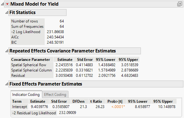
The Mixed Model report is shown in Figure 8.36. The fit statistics indicate not as good a fit as the isotropic (spatial structure) spherical model (AICc 240.54 compared to 234.08). The Repeated Effects Covariance Parameter Estimates report shows that the estimates for the Row (Spatial Spherical Row) and Column (Spatial Spherical Column) covariances are very close. There is no evidence to suggest that spatial correlations within rows and columns of the grid differ.
Figure 8.36 Mixed Model Report for Spatial Anisotropic Spherical Covariance Structure
 Determine the Type of the Spatial Structure
An isotropic spatial structure with no nugget is appropriate. To determine the type of the spatial structure, you can compare the available types.
1. Return to the Fit Model launch window.
2. Select the Repeated Structure tab.
3. Select Row and Column and click Repeated.
4. Select Spatial from the Structure list.
5. Select Power from the Type list.
6. Click Run.
Note the AICc and BIC values for the model fit.
7. Return to the Fit Model launch window.
8. Select Exponential from the Type list.
9. Click Run.
Note the AICc and BIC values for the model fit.
10. Return to the Fit Model launch window.
11. Select Gaussian from the Type list.
12. Click Run.
Note the AICc and BIC values for the model fit.
The observed AICc values for these types and the other fits that you performed are summarized in Table 8.2.
Structure | Type | AICc | BIC |
|---|---|---|---|
Spatial | Spherical | 234.08 | 240.16 |
Residual |
| 258.41 | 262.53 |
Spatial with Nugget | Spherical | 236.36 | 244.31 |
Spatial Anisotropic | Spherical | 240.54 | 248.50 |
Spatial | Power | 240.24 | 246.32 |
Spatial | Exponential | 240.24 | 246.32 |
Spatial | Gaussian | 238.37 | 244.44 |
The best fitting model (using the smallest AICc value) is the Spatial structure model with Spherical covariance structure. Next you compare this model to the complete and incomplete block models to complete the objectives of the uniformity trial.
 Compare the Model to Block Designs
1. Return to the Uniformity Trial data table.
2. In the Tables panel, run the Graph Builder script.
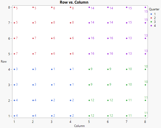
Figure 8.37 Graph Builder Plot of Proposed Complete and Incomplete Block Designs
This plot shows the proposed complete and incomplete block designs for the field. The color indicates the quarter fields that would serve as complete blocks. The numbered points represent the sub-quarter fields that would serve as incomplete blocks.
To fit the complete block model, follow these steps:
1. Return to the Fit Model launch window.
2. Select Repeated Structure tab.
3. Select Residual from the Structure list.
4. Remove Row and Column from the effect.
Otherwise, a pop-up window appears, stating, “Repeated columns and subject columns are ignored when the Residual covariance structure is selected.”
5. Select the Random Effects tab.
6. Select Quarter and click Add.
7. Click Run.
To fit the incomplete block model, follow these steps:
1. Return to the Fit Model launch window.
2. Select the Random Effects tab.
3. Select Quarter and click Remove.
4. Select Subquarter and click Add.
5. Click Run.
The following list shows both AICc and BIC values for the competing models. The spherical covariance structure results in the best model fit. This indicates that, for future studies using this field, a completely randomized design with spatially correlated errors is preferred.
• Spherical model (see Determine the Type of the Spatial Structure)
– AICc: 234.08
– BICc: 240.16
• Complete block (RCBD) model
– AICc: 259.90
– BICc: 265.97
• Incomplete block model
– AICc: 248.77
– BICc: 254.85
