Example of Analysis of Covariance with Equal Slopes
Use the Standard Least Squares personality of the Fit Model platform to fit an analysis of covariance model. An analysis of covariance model is a model with a primary factor of interest and a covariate term. The covariate is a factor that is not the primary factor of interest, but could impact the effect of the primary factor on the response. In this example, drug is the primary factor of interest and x is the covariate.
Note: This analysis assumes that the covariate impacts each level of the primary factor in a similar manner. That is, a covariance model with equal slopes. There is not an interaction term included in the model. For an unequal slopes model see Example of Analysis of Covariance with Unequal Slopes.
1. Select Help > Sample Data Folder and open Drug.jmp.
2. Select Analyze > Fit Model.
3. Select y and click Y.
4. Select both Drug and x and click Add.
5. Click Run.
Report sections are shown and described below.
Regression and Actual by Predicted Plots
Use the Regression and Actual by Predicted Plots to assess the model and to understand the impact of the covariate on the response.
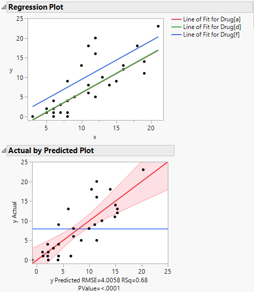
Figure 4.20 Plots for Analysis of Covariance with Equal Slopes
The Regression Plot shows that you have fit a model with equal slopes. The response increases with the covariate x at equal rates for each drug. Across the levels of the covariate x, the response is highest for Drug f.
Lack of Fit
The drug data table contains replicated observations. For example, rows 1 and 9 both have Drug = a and x = 11. When fitting models, replicated observations can be used to construct a pure error estimate of variation. Another estimate of error can be constructed for unspecified functional forms of covariates, or interactions of nominal effects. These estimates form the basis for a lack of fit test. If the lack of fit error is significant, this indicates that there is some effect in your data not explained by your model. See “Lack of Fit”.
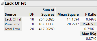
Figure 4.21 Analysis of Covariance with Equal Slopes Lack of Fit Test
The Lack of Fit report shows that the lack of fit error is not significant, as seen by the Prob > F value of 0.7507.
Least Squares Means
Use the least square means to compare the average response for each level of drug taking into account the covariate.
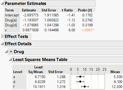
The least squares means differ from the ordinary means because they are adjusted for the effect of the covariate on the response. The least squares means are values that are predicted for each of the three levels of Drug, with the covariate, x, held at its mean value of 10.7333.
The least squares means are calculated using the parameter estimates given in the Parameter Estimates report:
Prediction Expression:
-2.696 - 1.185*Drug[a] - 1.0761*Drug[d] + 0.98718*x
For a:
-2.696 - 1.185*(1) -1.0761*(0) + 0.98718*(10.7333) = 6.71
For d:
-2.696 - 1.185*(0) -1.0761*(1) + 0.98718*(10.7333) = 6.82
For f:
-2.696 - 1.185*(-1) -1.0761*(-1) + 0.98718*(10.7333) = 10.16
Figure 4.22 Parameter Estimates and Least Square Means for Drug Test Data


