Example of Bagging to Improve Prediction
This example uses bagging through the Prediction Profiler. The goal is to improve predictions from a neural network model that simultaneously models four response variables as a function of three factors. Improving predictive power is one of a number of situations where bagging is used. Bagging is also especially helpful for unstable models.
Fit Neural Network Model
1. Select Help > Sample Data Folder and open Tiretread.jmp.
2. Select Analyze > Predictive Modeling > Neural.
3. Select ABRASION, MODULUS, ELONG, and HARDNESS and click Y, Response.
4. Select SILICA, SILANE, and SULFUR and click X, Factor.
5. Click OK.
6. (Optional) Enter 2121 next to Random Seed.
Note: Results vary due to the random nature of choosing a validation set in the Neural Network model. Entering the seed above enables you to reproduce the results shown in this example.
7. Click Go.
8. Click the red triangle next to Model NTanH(3) and select Save Formulas.
Note: This option saves the predicted values for all response variables from the neural network model to the data table. Later, these values are compared to the predictions that are obtained from bagging.
Perform Bagging
Now that the initial model has been constructed, you can perform bagging using that model. Access the Bagging feature through the Prediction Profiler.
1. Click the red triangle next to Model NTanH(3) and select Profiler.
The Prediction Profiler appears at the bottom of the report.
2. Click the Prediction Profiler red triangle and select Save Bagged Predictions.
3. Enter 100 next to Number of Bootstrap Samples.
4. (Optional) Enter 2121 next to Random Seed.
Note: Results vary due to the random nature of sampling with replacement. To reproduce the exact results in this example, set the Random Seed.
5. Click OK.
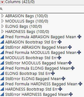
Return to the data table. For each response variable, there are three new columns denoted as Pred Formula <colname> Bagged Mean, StdError <colname> Bagged Mean, <colname> Bagged Std Dev. The Pred Formula <colname> Bagged Mean columns are the final predictions.
Figure 3.32 Columns Added to Data Table After Bagging
Compare the Predictions
To see how bagging improves predictive power, compare the predictions from the bagged model to the original model predictions. Use the Model Comparison platform to look at one response variable at a time.
1. Select Analyze > Predictive Modeling > Model Comparison.
2. Select Predicted ABRASION and click Y, Predictors.
3. Select Pred Formula ABRASION Bagged Mean and click Y, Predictors.
4. Click OK.
A window that contains a list of columns appears.
5. Select ABRASION and click OK.
6. Click the Model Comparison red triangle and select Plot Actual by Predicted.
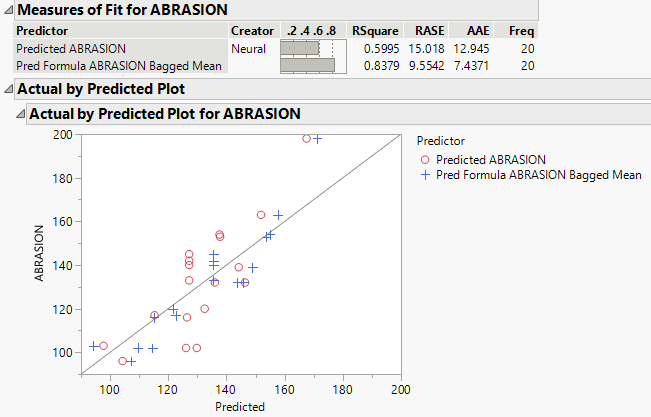
Figure 3.33 Comparison of Predictions for ABRASION
The Measures of Fit report and the Actual by Predicted Plot are shown in Figure 3.33. The predictions that were obtained from bagging are shown in blue. The predictions that were obtained from the original neural network model are shown in red. In general, the bagging predictions are closer to the line than the original model predictions. Because the bagging predictions are closer to the line, the RSquare value of 0.8379 for the bagged predictions is higher than the RSquare value for the original model predictions. You conclude that bagging improves predictions for ABRASION.
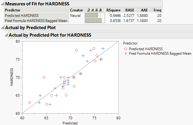
This example compared the predictions for ABRASION. To compare predictions for another response variable, follow step 2 through step 6, replacing ABRASION with the desired response variable. As another example, Figure 3.34 shows the Measures of Fit report for HARDNESS. The report shows similar findings as the Measures of Fit report for ABRASION. The RSquare value for the bagged predictions is slightly higher than the RSquare value for the original model predictions, which indicates a better fit and improved predictions.
Figure 3.34 Comparison of Predictions for HARDNESS


