Example of the ConstraintState Column Property
This example demonstrates the ConstraintState column property. It is based on an experiment presented in Snee (1979) and Piepel (1988), where there are boundary constraints on each factor and three additional linear constraints. In this example, you do the following:
1. Change one of the three additional constraints
2. Save the constraints to a table
3. Observe how the ConstraintState column property describes the direction of the inequality in the constraint
For further development of this example, see “An Extreme Vertices Example with Linear Constraints”.
1. Select Help > Sample Data Folder and open Design Experiment/Piepel.jmp.
2. In the Table panel, click the green triangle next to the DOE Dialog script.
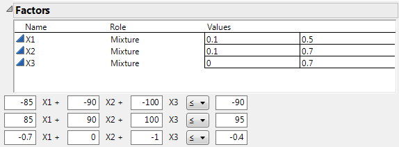
Notice the three linear constraints below the Factors section. To make the constraints more interpretable, you want to reformulate the first constraint in terms of a “greater than or equal to” inequality.
Figure A.35 Linear Constraints beneath Factors
3. In the first constraint, do the following:
– Type 85 next to X1.
– Type 90 next to X2.
– Type 100 next to X3.
– Select ≥ from the inequality menu.
– Type 90 to the right of the inequality sign.
4. Click the Mixture Design red triangle and select Save Constraints.
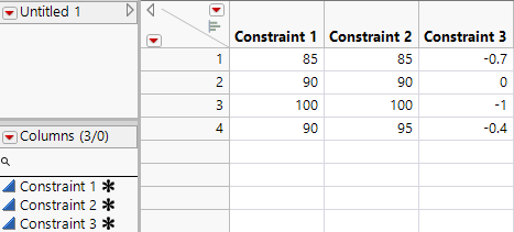
A table containing information about the constraints appears.
Figure A.36 Constraint Table
Each column contains the coefficients of the factors X1, X2, and X3 in rows 1 through 3. Row 4 contains the value that appeared to the right of the inequality sign.
5. Click the asterisk next to Constraint 1.
6. Click ConstraintState.
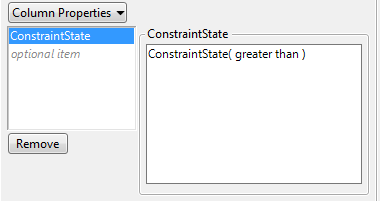
Figure A.37 ConstraintState Column Property Panel
The ConstraintState panel for X1 indicates that the direction of the inequality is “greater than” indicating greater than or equal to ≥.
7. Click Cancel.


