Example of an Extreme Vertices Design

Use the Mixture Design platform to create extreme vertices designs. An extreme vertices design requires restricted ranges on one or more of the factors, as defined by limits in the Factors panel or by linear constraints. The design consists of mixtures at the vertices of the factor space and at the averages of vertices up to a specified degree. The centroid point for two neighboring vertices joined by a line is a second-degree centroid. The centroid point for vertices sharing a plane is a third-degree centroid.

An Extreme Vertices Example with Range Constraints

1. Select DOE > Classical > Mixture Design.

2. Under Factors, enter 2 for the number of additional factors to add and click Add.

3. Set the ranges for the five factors as shown in Figure 14.11 and click Continue.

Figure 14.11 Ranges for Five-factors 

4. Enter 4 in the Degree text box and click Extreme Vertices.

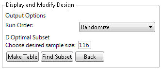
Figure 14.12 Display and Modify Panel for Extreme Vertices Example 

The default number of runs for this five-factor, degree 4 extreme vertices design is 116. This is the number of extreme vertices and averages up to degree 4 for these five factors given the constraints on their ranges. JMP uses the default set of mixtures as a candidate set to generate a smaller D Optimal design.

5. (Optional) To match the output of this example, click the Mixture Design red triangle and select Set Random Seed, and then enter 1409.

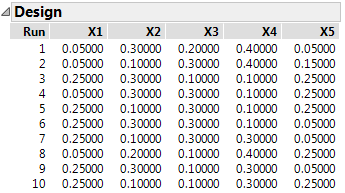
6. Enter 10 in the Choose desired sample size box and click Find Subset to generate the design.

Note: The Find Subset option uses the row exchange method (not coordinate exchange) to find the optimal subset of rows.

Figure 14.13 Ten Run D-optimal Extreme Vertices Design 

7. Click Make Table.

Visualize the Design

8. From the design table, select Graph >Ternary Plot.

9. Select X1, X2, X3, X4, and X5 and click X, Plotting, and then click OK.

Figure 14.14 Partial Output of Ternary Plot for Five-Factor Design 

When you have more than three mixture components, the ternary plot shows a series of plots. Each plot has two component axes and the third axis is the sum of all other components. The plots are shaded if you have a constrained region. The unshaded portion represents the feasible region. For more information about ternary plots, see Ternary Plot Overview.

An Extreme Vertices Example with Linear Constraints

Consider the classic example presented by Snee (1979) and Piepel (1988). This example has three factors, X1, X2, and X3, with factor bounds and three linear constraints.

To create an extreme vertices design for this example:

1. Select DOE > Classical > Mixture Design.

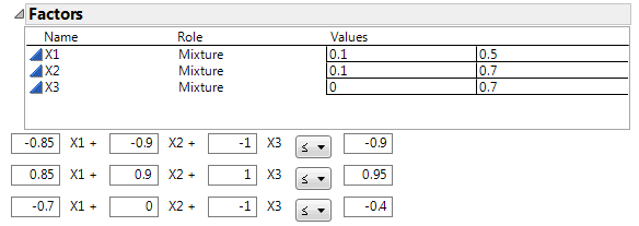
2. Enter the values from Figure 14.15 for X1, X2, and X3 and click Continue.

Figure 14.15 Values and Linear Constraints for the Snee and Piepel Example 

3. Click Linear Constraint three times. Enter the constraints as shown in Figure 14.15.

4. Click the Extreme Vertices button.

5. Click Make Table.

Visualize the Design

6. From the design table, select Graph >Ternary Plot.

7. Select X1, X2, and X3 and click X, Plotting, and then click OK.

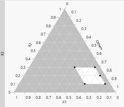
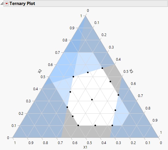
Figure 14.16 Ternary Plot Showing Piepel Example with Constraints 

The ternary plot shows the feasible region as defined by the factor limits and the linear constraints. The design points are at the six vertices of the feasible region, at the six edge mid-points, and the overall centroid. For more information about ternary plots, see Ternary Plot Overview.