Example of the Mixture Column Property
Use the Mixture column property to evaluate a mixture design. The data are based on an example from Atkinson and Donev (1992). The design includes three mixture factors and one non-mixture factor:
• The response is the electromagnetic Damping of an acrylonitrile powder.
• The three mixture ingredients are copper sulphate (CuSO4), sodium thiosulphate (Na2S2O3), and Glyoxal.
• The non-mixture environmental factor of interest is the Wavelength of light.
Though Wavelength is theoretically continuous, the researchers were interested only in predictions at three discrete wavelengths. As a result, Wavelength is treated as a categorical factor with three levels.
For more information about using Custom Design to construct a design for this situation, see “Examples of Mixture Experiments”.
1. Select Help > Sample Data Folder and open Design Experiment/Donev Mixture Data.jmp.
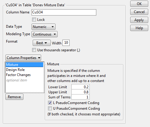
2. Click the asterisk next to CuSO4 in the columns panel and select Mixture.
Figure A.20 Mixture Column Property Panel for CuSO4
Notice the following:
– The Lower Limit is 0.2, the minimum design setting for CuSO4.
– The Upper Limit is 0.8, the maximum design setting for CuSO4.
– The Sum of Terms is set to 1. This is the sum of the three mixture factors.
– The L PseudoComponent Coding option is selected. See PseudoComponent Coding.
3. Click Cancel.
4. Click the asterisk next to Glyoxal in the columns panel and select Mixture.
For this factor, note the following:
– The Lower Limit is 0, the minimum design setting for Glyoxal.
– The Upper Limit is 0.6, the maximum design setting for Glyoxal.
5. Click Cancel.
6. In the Donev Mixture Data.jmp data table, click the green triangle next to the Model script.
The model contains the main effects of the mixture factors and two-way interactions for all four factors.
7. Click Run.
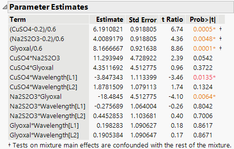
In the Parameter Estimates report, the mixture factors appear in their pseudo-component coded form. When the mixture factors appear in interactions, they are not denoted in coded form. Nevertheless, the model fitting is based on the pseudo-components. The first three terms in the Parameter Estimates report (Figure A.21), show the coded form for the mixture factors.
Figure A.21 Parameter Estimates Report
8. Click the Response Damping red triangle and select Estimates > Show Prediction Expression.
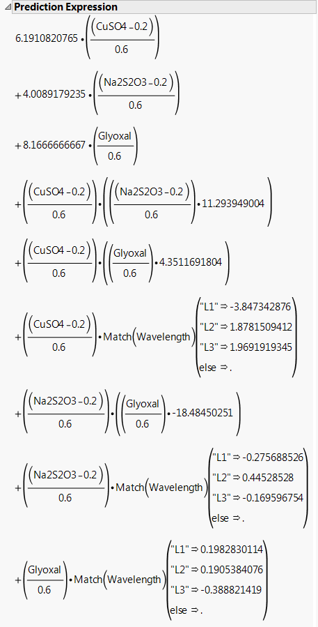
The Prediction Expression report shows the model that was fit. Note that the mixture factors are transformed using the L PseudoComponent coding.
Figure A.22 Prediction Expression for Damping Model
Suppose that you are interested in predictions at Wavelength L2. Suppose also that Na2S2O3 and Glyoxal are set to their low values, 0.2 and 0 respectively, and that CuSO4 is set to its high value, 0.8. In this case, the predicted Damping equals the parameter estimate for CuSO4 (6.191) plus the parameter estimate for CuSO4*Wavelength[L2] (1.878). You can verify this in the Prediction Profiler.
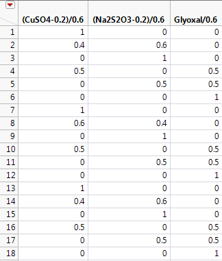
9. Click the Response Damping red triangle and select Save Columns > Save Coding Table.
Figure A.23 First Three Columns of Coding Table Showing Coded Mixture Factors
For this particular design, the L Pseudo Component coding transforms the mixture factors to range between 0 and 1. Note that this does not happen in general


