Prediction Graph

In the Degradation platform, use the Prediction Graph tab to predict the Y variable for a specified Time value.

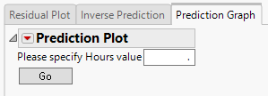
Figure 16.15 Prediction Plot Tab 

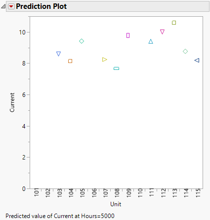
For the GaAs Laser example, no data was collected after 4000 hours. If you want to predict the percent increase in operating current after 5000 hours, enter 5000 and click Go. A plot is produced showing the estimated percent decrease after 5000 hours for all the units.

Figure 16.16 Prediction Plot 

The Prediction Plot red triangle menu contains the following options:

Save Predictions

Saves the predicted response values for the current model to a new data table. The table also includes columns for lower and upper bounds based on the setting of the Longitudinal Prediction Interval option.

Longitudinal Prediction Interval

Shows or hides confidence or prediction intervals for the estimated responses that are shown on the Prediction Plot. When intervals are enabled, the intervals are also included in the data table that is created when using the Save Predictions option.

Longitudinal Prediction Time

Specifies the time value for which you want to predict the response.

Longitudinal Prediction Alpha

Specifies the alpha level that is used for the intervals in the Prediction Plot.