Simulation Settings for Factors
By default, factors (inputs) in the Simulator are defined by the functions that you select when you launch a profiler. There are options for changing the location, error, and noise that enable you to modify how your factors are simulated.
Fixed
Fixes the factor at the current value in the profiler for all simulation runs.
Random
Draws a random value of the factor for each simulation run from the specified distribution and distributional parameters. When you select Random, distribution options appear. For more information about the options, see Continuous Factors and Categorical Factors.
Note: The default random distribution is a normal distribution with a mean at the current factor setting and a standard deviation estimated by the range of the factor divided by 5. The mean of the normal distribution is automatically updated if you change the factor setting in the profiler. There are other random distributions that also update parameters automatically when the factor settings are changed. The Triangular distribution updates all three parameters, the Cauchy distribution updates the mode, and the Johnson Su distribution updates θ.
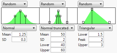
Figure 8.5 Example of Three Random Distributions
Expression
Generates values for the factor based on a JSL expression. This gives you flexibility to use a random distribution of your choice. For example, you could create a censored normal distribution that guaranteed nonnegative values with an expression such as the following:
Max(0,RandomNormal(5,2))After entering the expression, click the Reset button to submit the expression.
Multivariate
Generates values for the factor based on a multivariate normal distribution. Specify the mean and standard deviation for each factor. The correlation matrix is defined separately in the X Correlation Specification report. You can use this option to accommodate correlated factors.
Figure 8.6 Defining a Correlation Matrix for the Multivariate Option
Tip: To specify the same setting for all of the factors, press Ctrl and select the desired setting.
Continuous Factors
For continuous factors the random distributions available use standard random functions that are described in “Random Functions” in Using JMP. Descriptions of the specialized distributions available follow:
Normal weighted
Generates values from a weighted normal distribution with the given mean and standard deviation. The weighting is a specific sampling scheme used to simulate rare events from the tails of the distribution. This is a good choice when you want to simulate very low defect rates. See Statistical Details for the Simulator.
Normal truncated
Generates values from a normal distribution limited by lower and upper limits. Any randomly generated value that exceeds a limit is discarded and another value is generated. This is a good choice when you want to simulate an inspection system where inputs that do not satisfy specification limits are discarded.
Normal censored
Generates values from a normal distribution limited by lower and upper limits. Any randomly generated value that exceeds a limit is set to that limit, putting a density mass at the limits. This is a good choice when you want to simulate systems where inputs that do not satisfy specification limits are reworked until they are at the specification limit.
Sampled
Generates factor values by selecting a value at random from that factor’s column in the data table.
External
Generates factor values by selecting a value at random from a column in another table. You are prompted to choose the table and column.
Tip: To specify the same distribution for all of the factors, press Ctrl and select the desired distribution.
Note: The Aligned check box appears when you select Sampled or External. It is used when two or more factors are set to Sampled or External. When checked, the random draws come from the same row of the table. This maintains the correlation structure between two columns. If the Aligned option is used to associate two columns in different tables, the columns must have the same number of rows.
Categorical Factors
For a categorical factor the random distribution is characterized by probabilities specified for each category. By default, the probabilities are set to the observed probabilities in the data table. You can change the probabilities using the handles in the plot or by changing the numerical values in the Prob column. The probabilities must sum to 1.
Note: If the probabilities that you select do not sum to 1, they are automatically regularized to sum to 1 once you click the Simulate button.
When the simulation for a factor is set to Random, a graphical representation of the random distribution density is shown. The graph shows the form of the density for the continuous distributions, and provides control points that can be dragged to change the distribution. The drag points for the Normal are the mean and the mean plus or minus one standard deviation. The Normal truncated and censored add points for the lower and upper limits. The Uniform and Triangular have limit control points, and the Triangular adds the mode.
Mixture Factors
For mixture factors there are two random distributions available. Mixture factors must be generated from the same random distribution. However, there can be a combination of fixed and random mixture factors.
Mixture Uniform
Generates random uniform points over a convex polytope, given the specified lower and upper bounds for each factor. This ensures that each generated row upholds the mixture constraints. This option uses the Polytope Uniform Random JSL function. See “Utility Functions” in the JSL Syntax Reference.
Mixture Dirichlet
Generates random points from a Dirichlet distribution with the specified α parameter for each factor. The probability density function of the Dirichlet distribution is calculated as follows:

where B(α) is the multivariate beta function, which acts as a normalizing constant. The Mixture Dirichlet option is available only if the bounds on the factors create a mixture region that is a simplex, or generalized triangle.

