Associative Arrays in Graph Theory
In JSL, you can use associative arrays for graph theory data structures, such as the following directed graph example:
g = Associative Array();
g[1] = Associative Array({1, 2, 4});
g[2] = Associative Array({1, 3});
g[3] = Associative Array({4, 5});
g[4] = Associative Array({4, 5});
g[5] = Associative Array({1, 2});
This is a two-level associative array. The associative array g contains five associative arrays (1, 2, 3, 4, and 5). In the containing array g, both the keys (1-5) and the values (the arrays that define the map) are important. In the inner associative arrays, the values do not matter. Only the keys are important.
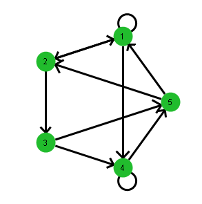
The associative array represents the graph shown in Figure 7.2:
• node 1 is incident on nodes 1, 2, and 4
• node 2 is incident on nodes 1 and 3
• node 3 is incident on nodes 4 and 5
• node 4 is incident on nodes 4 and 5
• node 5 is incident on nodes 1 and 2
Figure 7.2 Example of a Directed Graph
The following depth-first search function can be used to traverse this graph, or any other directed graph represented as an associative array:
dfs = Function( {ref, node, visited}, {chnode, tmp},Write( "\!NNode: ", node, ", ", ref[node] << Get Keys );
visited[node] = 1;tmp = ref[node];
chnode = tmp << first;While( !Is Missing( chnode ),
If( !visited[chnode], visited = Recurse( ref, chnode, visited ));
chnode = tmp << Next( chnode ););
visited;
);
Notes:
• The first argument is the associative array that contains the map structure.
• The second argument is the node that you want to use as the starting point.
• The third argument is a vector that the function uses to keep track of nodes visited.
To see how the preceding example works, add the following expression to the end of the script:
dfs( g, 2, J( N Items( g << Get Keys ), 1, 0 ) );
Here is the output:
Node 2: {1, 3}
Node 1: {1, 2, 4}
Node 4: {4, 5}
Node 5: {1, 2}
Node 3: {4, 5}
[1, 1, 1, 1, 1]
The first five output lines show that starting from node 2, you can reach all the other nodes in the order in which they are listed. Each node also lists the nodes it is incident on (the keys). The value for each key is 1. The final line is a matrix that shows that you can reach each node from 2. If there were nodes that could not be reached from node 2, their values in the matrix would be 0.
Here is how to read the traversal of the nodes:
1. Start at node 2 and go to node 1.
2. From node 1, go to node 4.
3. From node 4, go to node 5.
4. From node 5, go back to node 2, and then to node 3.
Map Script
Here is the script that produced the map shown in Figure 7.2.
New Window( "Directed Graph",
Graph Box(Frame Size( 300, 300 ),
X Scale( -1.5, 1.5 ),
Y Scale( -1.5, 1.5 ),
Local( {n = N Items( g ), k = 2 * Pi() / n, r, i, pt, from, to,
edge, v, d},
Fill Color( "green" );
Pen Size( 3 );
r = 1 / (n + 2);
For( i = 1, i <= n, i++,
pt = Eval List( {Cos( k * i ), Sin( k * i )} );
edges = g[i];
For( edge = edges << First, !Is Empty( edge ),
edge = edges << Next( edge ),to = Eval List( {Cos( k * edge ), Sin( k * edge )} );
If( i == edge,
// elseCircle( Eval List( 1.2 * pt ), 0.9 * r ),
v = pt - to;
d = Sqrt( Sum( v * v ) );
{from, to} = Eval List( {pt * (d - r) / d + to * r / d, pt * r / d + to *(d - r) / d}
);
Arrow( from, to ););
);
Circle( pt, r, "fill" );
Text( Center Justified, pt - {0, 0.05}, Char( i ) );
);
)
)
);
