Choose a Design
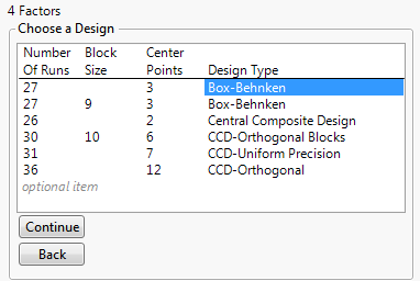
In the Response Surface Design platform, the Choose Design section enables you to select a design. The designs include two types:
Figure 12.13 Choose a Design Panel for Four Factors
Box-Behnken Designs
Box-Behnken designs have only three levels for each factor and have no design points at the vertices of the cube defined by the ranges of the factors. These designs can be useful when it is desirable to avoid extreme settings for engineering considerations. However, these designs result in higher prediction variance near the vertices than do central composite designs.
Central Composite Designs
Central composite designs have center points and axial points. An axial point is a point where one factor is set to a high or low value (an axial value) and all other factors are set to the midrange, or center, value.
A central composite design can have axial points that fall beyond the faces of the hypercube defined by the specified factor ranges. This means that each factor might require five distinct settings, including two that fall beyond the range of values specified in the Factors section. However, JMP enables you to place design points on the face.
The default number of center points that JMP recommends are based on the type of design. The center points are based on the goals and optimality criteria for the design. The number of center points can impact the uniform precision or orthogonality properties of the design.
The following types of central composite designs are available:
Central Composite Design
The typical central composite design for defining a response surface model. Uses two center points.
CCD-Uniform Precision
A design where the number of center points is chosen so that the prediction variance near the center of the design space is very flat. These designs use a large number of center points.
CCD-Orthogonal
A design where the number of center points and the axial values are chosen so that the second-order parameter estimates are minimally correlated with the other parameter estimates. These designs use a large number of center points.
CCD-Orthogonal Blocks
A design where the second-order parameter estimates and block effects are minimally correlated with the other parameter estimates. These designs use a large number of center points.
Axial Value
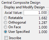
When you select a central composite design and then click Continue, you have the option to provide axial scaling information. In placing axial values, the values shown are used to multiply half of the specified range of a factor. If you specify a value of 1.0 next to Axial Value, then axial points in the resulting design are placed on the faces of the cube defined by the factors. You can set the axial value according to the following options:
Figure 12.14 Axial Value Panel
Rotatable
The prediction variance depends only on the scaled distance from the center of the design. The axial points are more extreme than the factor ranges. The axial points are set at the 4th root of the number of factorial runs.
Orthogonal
The effects are not correlated with each other, so the estimates have the smallest standard errors and shortest confidence intervals. The axial points are more extreme than the factor ranges. The axial points are determined by the following calculation:

where
nf = number of factorial runs
ns = number of axial runs
nc = number of center runs
On Face
Places the axial points at the extremes of the specified factor ranges. This results in three factor levels. This is a practical choice but the resulting design is not orthogonal or rotatable.
User Specified
Places the axial points at a distance specified by the value that you enter in the Axial Value text box. This enables the choice of axial values based on practical constraints on the factor levels. The resulting design is unlikely to be orthogonal or rotatable.
Inscribe
Rescales the design so that the axial points are at the low and high ends of the factor range. The factorial design points are shrunken based on that scaling.

