Clip Display Segs in Graphics
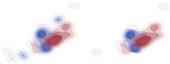
Display segs (such as reference lines, grid lines, and contours) in JMP graphs can be clipped to conform to the natural boundaries of the underlying data. This gives you a better view of the boundaries. For example, Figure 12.29 shows contours that are clipped to the boundaries of a map of the United States.
Figure 12.29 Unclipped (Left) and Clipped (Right) Boundaries
Send the Clip Shape message to the Contour Seg object to clip the display segs.
Open( "$SAMPLE_DATA/Cities.jmp" );
gb = Graph Builder(Size( 653, 396 ),
Show Control Panel( 0 ),Variables( X( :Longitude ), Y( :Latitude ) ),
Elements( Contour( X, Y, Legend( 2 ) ) ),
SendToReport(
Dispatch(
{}, "Graph Builder",FrameBox,
{Background Map( Boundaries( "US States" ) ), Grid Line Order( 2 ), Reference Line Order( 3 )})
)
);
cs = (gb << Report)[FrameBox( 1 )] << Find Seg( Contour Seg( 1 ) );
Wait( 2 );
cs << Clip Shape( Boundaries( "US States" ) );
Tip: Clip Shape(Empty()) removes the clipping path.
Here’s an example of defining the clip shape path with a matrix:
Open( "$SAMPLE_DATA/Big Class.jmp" );
gb = Graph Builder( Show Control Panel( 0 ),Variables( X( :height ), Y( :weight ), Overlay( :sex ) ),
Elements( Contour( X, Y, Legend( 3 ) ) )
);
r = ( gb << Report );cs = r[FrameBox( 1 )] << Find Seg( Contour Seg( 1 ) );
cs << Clip Shape( Path( [60 80 1, 50 140 2, 65 120 2, 70 65 -2] ) );
Figure 12.30 Unclipped (Left) and Clipped (Right) Contours
The matrix [60 80 1, 50 140 2, 65 120 2, 70 65 -2] indicates the following:
1. Start at 60, 80.
2. Draw a line to 50, 140.
3. Draw a line to 65, 120.
4. Draw a line to 70, 65.
5. Connect back to the first point.

