Example of a Box-Cox Transformation
In this example, you compare two time series analyses. In one analysis, you use a Box-Cox transformation and in the other, you analyze a manually transformed time series. When the lambda value is set to zero, the Box-Cox transformation is an approximate log transformation. However, using the Box-Cox transformation for the analysis makes the results easier to interpret since all forecasts are transformed back and reported on the original scale.
1. Select Help > Sample Data Folder and open Time Series/Seriesg.jmp.
2. Select Analyze > Specialized Modeling > Time Series.
3. Select Passengers and click Y, Time Series.
4. Select Time and click X, Time ID.
5. Select Use Box-Cox Transformation.
Use the default value of 0 for Lambda.
6. Click OK.
7. Click the red triangle next to Time Series Box-Cox Transformed Passengers and select Seasonal ARIMA.
8. In the ARIMA section of the Seasonal ARIMA Specification window, set the following parameters.
– Set p, Autoregressive Order to 0.
– Set d, Differencing Order to 1
– Set q, Moving Average Order to 1
9. In the Seasonal ARIMA section of the Seasonal ARIMA Specification window, set the following parameters.
– Set P, Autoregressive Order to 0
– Set D, Differencing Order to 1
– Set Q, Moving Average Order to 1
10. Deselect Intercept to run a model without an intercept.
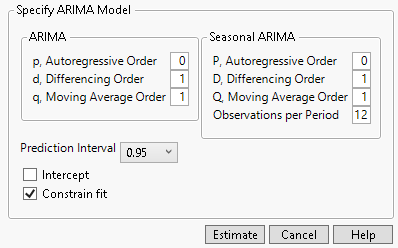
Your window should now match the window shown in Figure 18.22.
Figure 18.22 Seasonal ARIMA Specifications
11. Click Estimate.
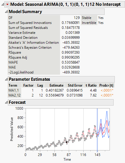
Figure 18.23 Seasonal ARIMA Model for Box-Cox Transformed Passengers Data
The parameter estimates are equivalent to those obtained from running the same model on the Log Passengers column. However, the forecasts and prediction intervals in Figure 18.23 are on the original scale.

