Example of a Plackett-Burman Design
Use the Screening Design platform to construct a 12-run Plackett-Burman design for five factors. To facilitate completing the Screening window, use the Load Responses and Load Factors commands.
Create the Plackett-Burman Design
1. Select DOE > Classical > Factor Screening > Screening Design.
2. Select Help > Sample Data Folder and open Design Experiment/Reactor Response.jmp.
3. Click the Screening Design red triangle and select Load Responses.
4. Select Help > Sample Data Folder and open Design Experiment/Reactor Factors.jmp.
5. Click the Screening Design red triangle and select Load Factors.
The Load Responses and Load Factors commands fill in the Responses and Factors sections with the response and factor names, goal and limits for the response, and values for the factors. See Figure 10.14 for the completed Responses and Factors sections.
6. Click Continue.
Note: Setting the random seed in the next step reproduces the run order shown in this example. In constructing a design on your own, this step is not necessary.
7. (Optional) Click the Screening Design red triangle, select Set Random Seed, type 34567, and click OK.
8. From the Choose Screening Type panel, accept the default selection to Choose from a list of fractional factorial designs and click Continue.
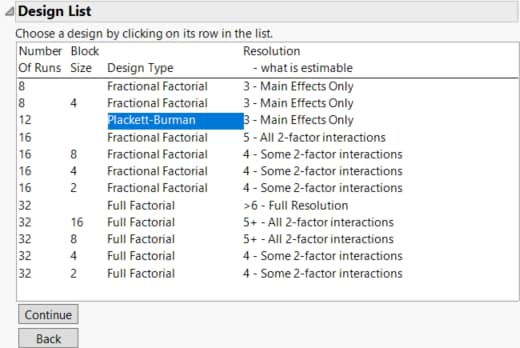
9. Select the Plackett-Burman design.
Plackett-Burman designs with run sizes that are not a power of two tend to have complex aliasing structures. In particular, main effects can be partially aliased with several two-way interactions. See Evaluate the Design. Notice that the 12-run Plackett-Burman design is designated as having Resolution 3.
Figure 10.21 Design List Showing Plackett-Burman Screening Design
10. Click Continue.
11. Click Make Table.
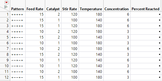
Figure 10.22 Design Table for Placket-Burman Design
A column called Percent Reacted is included in the design table. You should conduct your experimental runs in the order shown in the table, recording your results in the Percent Reacted column.
Evaluate the Design
1. Return to your Screening Design window. If you have closed this window, run the DOE Dialog script in your design table.
2. Open the Design Evaluation > Color Map on Correlations section.
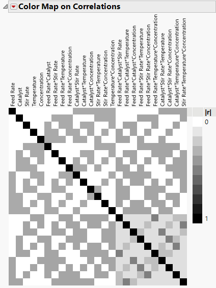
Figure 10.23 Color Map for Absolute Correlations
The diagonal cells have correlations of one, as expected. White cells correspond to effects that have correlations equal to 0. The gray and black cells correspond to effects that have correlations greater than zero. Hover over cells to see the effects involved and their absolute correlations. For example, notice that Feed Rate is correlated with several two-way and three-way interactions.
Note: The color map from the screening design contains 3-way interactions for designs with 8 or fewer factors. The color map from the design evaluation script contains up to 2-way interactions.
3. Open the Alias Matrix.
Figure 10.24 Alias Matrix - Partial View Showing Up to Two-Way Interactions
Because the design is orthogonal for the main effects, the Alias Matrix gives the numerical values of the correlations between effects. See Alias Matrix. For example, notice that Feed Rate is partially aliased with six two-way interactions and with four three-way interactions. These are the interactions corresponding to the entries of 0.333 and -0.33 in the row for Feed Rate.
Analyze the Results
The data table Plackett-Burman.jmp contains the results of the designed experiment. Recall that you suspect that the Temperature*Concentration interaction is active. You proceed under the assumption that this is the only potentially active interaction.
1. Select Help > Sample Data Folder and open Design Experiment/Plackett-Burman.jmp.
2. Run the Model script by clicking the icon to its left.
3. Select Temperature in the Select Columns list and Concentration in the Construct Model Effects list.
4. Click Cross.
5. Click Run.
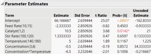
Figure 10.25 Parameter Estimates for Full Model
The Actual by Predicted Plot indicates no lack of model fit. The Parameter Estimates report shows that Catalyst is significant at the 0.05 level and that the Concentration*Temperature interaction is almost significant at the 0.10 level.
Reduce the Model
You want to identify those effects that have the most impact on the response. To see these active effects more clearly, remove insignificant effects using the Effect Summary section.
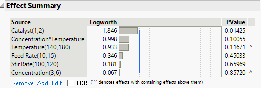
Figure 10.26 Effect Summary for Full Model
Although Concentration is the least significant effect, it is involved in a higher-order interaction (Concentration*Temperature), as indicated by the caret to the right of its PValue. Based on the principle of effect heredity, Concentration should not be removed from the model while the Concentration*Temperature interaction remains in the model. See Effect Heredity. The next least significant effect is Stir Rate.
1. In the Effect Summary section, select Stir Rate and click Remove.
Feed Rate is the next least significant effect that can be removed.
2. In the Effect Summary section, select Feed Rate and click Remove.
Figure 10.27 Effect Summary for Reduced Model
The PValue column indicates that the Catalyst main effect and the Concentration*Temperature interaction are both significant at the 0.05 level. The model should not be reduced any further. If all other interactions are inactive or negligible, then you can conclude that Catalyst and the Concentration*Temperature interaction are active effects.
