Example of a Power Analysis
In this example, you are interested in the power of your design to detect effects of various magnitudes on your response, Strength. The design has three continuous factors, one two-level categorical factor, and a three-level categorical factor. The three-level categorical factor was a blocking factor in the original design.
1. Select Help > Sample Data Folder and open Design Experiment/Coffee Data.jmp.
2. Select DOE > Design Diagnostics > Evaluate Design.
3. Select Grind, Temperature, Time, Charge, and Station and click X, Factor.
You can also add Strength as Y, Response. However, specifying the response has no effect on the properties of the design.
4. Click OK.
5. Click the gray disclosure icon to open the Power Analysis section. Note that the Significance Level is set to 0.05.
6. Enter 0.1 as the Anticipated RMSE. This is your estimate of the standard deviation of Strength for fixed design settings.
You are interested in the effect of Station on Strength.
Anticipated Coefficients
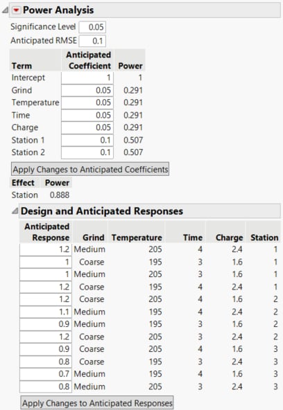
To estimate power, you need to set the anticipated coefficients that would yield the difference that you are interested in detecting. For example, Temperature is a continuous factor with coded levels of -1 and 1. Consider the test whose null hypothesis is that Temperature has no effect on Strength. Figure 16.14 shows that the power of this test to detect a difference of 0.10 (=2*0.05) units across the levels of Temperature is only 0.291.
1. To estimate the power to detect a change of 0.10 units in strength as you vary Temperature, Time, or Charge from their low to high levels, set the anticipated coefficient for each factor to 0.05. A change from low to high is two coded units.
2. To estimate the power to detect a change of 0.10 units in strength as you vary Grind from Coarse to Medium, set the anticipated coefficient for Grind to 0.05. A change from Coarse to Medium is two coded units.
3. To estimate the power to detect a change of 0.10 units in strength as you vary Station, set the anticipated coefficients for Station 1 and Station 2 to 0.10. Since Station is a three-level categorical factor, it is represented by two terms in the Parameters list: Station 1 and Station 2. An increase due to each of Stations 1 and 2 of 0.10 units beyond the overall anticipated mean corresponds to a decrease due to Station 3 of 0.20 units from the overall anticipated mean.
4. Click Apply Changes to Anticipated Coefficients. The Anticipated Response values are updated to reflect the coefficients that you have specified.
Figure 16.14 Completed Power Analysis
For the first four factors in the power analysis table, the test that the factor has no effect on Strength has a power of 0.291 to detect a difference of 0.10 (=2*0.05) units across the levels of each factor.
The power for the whole Station effect, 0.888, is provided below the power table. Since Station is a three-level categorical factor the powers in the power analysis table are partial power values. Note that the test that Station has no effect on Strength is an F test.
