Example of an Arrhenius Accelerated Failure Lognormal Model
In this example, use the Fit Parametric Survival platform to fit a distribution to the failure times of units that are stressed by heating. This stress causes the units to fail faster so that enough failures are obtained.
1. Select Help > Sample Data Folder and open Reliability/Devalt.jmp.
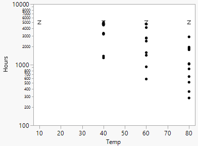
First, use the Bivariate platform to see a plot of hours by temperature using the log scale for time.
2. Select Analyze > Fit Y by X.
3. Select Hours and click Y, Response.
4. Select Temp and click X, Factor.
5. Click OK.
Figure 15.7 Bivariate Plot of Hours by Log Temp
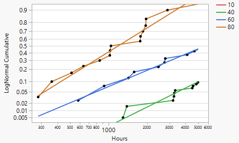
Next, use the Survival platform to produce a lognormal plot of the data for each temperature.
6. Select Analyze > Reliability and Survival > Survival.
7. Select Hours and click Y, Time to Event.
8. Select Censor and click Censor.
9. Select Temp and click Grouping.
10. Select Weight and click Freq.
11. Click OK.
12. Press Alt and click the red triangle next to Product-Limit Survival Fit.
Tip: The Alt key enables you to make multiple red triangle menu selections simultaneously.
13. Select LogNormal Plot and LogNormal Fit.
14. Click OK.
Figure 15.8 Lognormal Plot
Next, use the Fit Parametric Survival platform to fit one model using an effect for temperature.
15. Select Analyze > Reliability and Survival > Fit Parametric Survival.
16. Select Hours and click Time to Event.
17. Select x and click Add.
18. Select Censor and click Censor.
19. Select Weight and click Freq.
20. Change the Distribution type to Lognormal.
21. Click Run.
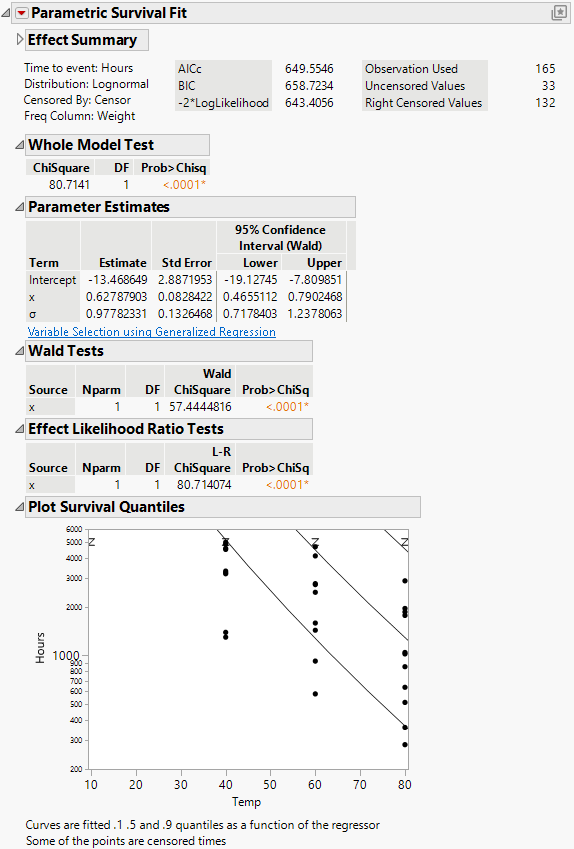
Figure 15.9 Devalt Parametric Output
The result shows the regression fit of the data:
– If there is only one effect and it is continuous, then a plot of the survival as a function of the effect is shown. Lines are at 0.1, 0.5, and 0.9 survival probabilities.
– If the effect column has a formula in terms of one other column, as in this case, the plot is done with respect to the inner column. In this case, the effect was the column x, but the plot is done with respect to Temp, of which x is a function.
Finally, get estimates of survival probabilities extrapolated to a temperature of 10 degrees Celsius for the times 30000 and 10000 hours.
22. Click the Parametric Survival Fit red triangle and select Estimate Survival Probability.
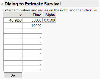
23. Enter the values shown in Figure 15.10 into the Dialog to Estimate Survival.
The Arrhenius transformation of 10 degrees is 40.9853, the effect value.
Figure 15.10 Estimating Survival Probabilities
24. Click Go.
Figure 15.11 Survival Probabilities
The Estimates of Survival report shows the estimates and a confidence interval.


