Example of Analyzing a Full Factorial Design
Use two methods to analyze results from a full factorial design. This example demonstrates screening and stepwise regression, as well as how to use the Prediction Profiler.
Analysis Using Screening Platform
1. Select Help > Sample Data Folder and open Design Experiment/Reactor 32 Runs.jmp.
2. Run the Screening script.
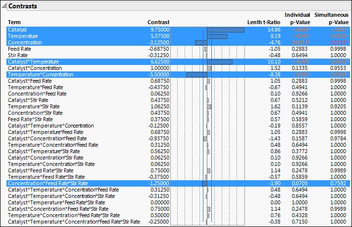
The Screening report shows a Contrasts report and a Half Normal Plot. The Contrasts report shows estimates for all 31 potential effects, up to the five-way interaction.
Figure 13.4 Contrasts Report for Reactor 32 Runs.jmp
Note: Because the p-values in the Contrasts report are obtained using a Monte Carlo simulation, you might not obtain the same values as shown in Figure 13.4. See Statistical Details for Lenth’s Pseudo-Standard Error.
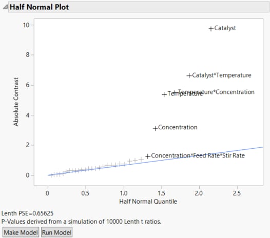
The six highlighted effects in the Contrasts section are labeled in the Half Normal Plot.
Figure 13.5 Half Normal Plot for Reactor 32 Runs.jmp
The Half Normal Plot provides strong evidence that at least five of the labeled effects are larger than would be expected if they were the result of random variation. This suggests that these effects are active. The plot does not provide a clear indication that the three-way Concentration*Feed Rate*Stir Rate interaction is active.
In the Contrasts section in Figure 13.4, the Individual p-Value for the three-way Concentration*Feed Rate*Stir Rate interaction is 0.0705 and its Simultaneous p-Value is 0.7592. Because the effect does not stand out on the Half Normal Plot and because its p-values are large, you decide not to include this effect in your model.
3. In the Half Normal Plot, drag a rectangle to select all labeled effects except for Concentration*Feed Rate*Stir Rate.
4. Click Make Model to open a Fit Model window containing the five effects.
5. Click Run.
The Actual by Predicted plot shows no evidence of lack of fit and the Effect Summary section shows that all five effects are significant.
Analysis Using Stepwise Regression
1. Return to the Reactor 32 Runs.jmp data table, or reopen it by selecting Help > Sample Data Folder and opening Design Experiment/Reactor 32 Runs.jmp.
2. Run the Model script.
The Construct Model Effects list contains only up to two-way interactions. You want to consider all interactions.
3. From the Select Columns list, select Feed Rate through Concentration.
4. Click Macros > Full Factorial.
All possible effects are added in the Construct Model Effects list.
5. Change the Personality to Stepwise.
6. Click Run.
7. Change the Stopping Rule to Minimum AICc.
For designed experiments, AICc is preferred to BIC. This is because BIC is typically a more lenient stopping rule than AICc as it tends to allow inactive effects into the model.
8. Click Go.
The Stepwise procedure selects six effects as potentially active.
9. Click Run Model.
This fits a model using the six effects. The Effect Summary section indicates that Catalyst*Concentration is not significant at the 0.05 significance level as the p-value is 0.0896.
10. Select Catalyst*Concentration in the Effect Summary section and click Remove.
The five remaining effects are all highly significant. These are the same five effects that you identified using the Screening platform (Analysis Using Screening Platform).
Optimal Settings Using the Prediction Profiler
Now, find optimal settings for the three active factors involved in the five significant effects that you retained in your model.
1. In the Reactor 32 Runs.jmp data table, run the Reduced Model script.
The Reduced Model script opens a Fit Model window for the five-effect model that you identified in Analysis Using Screening Platform and Analysis Using Stepwise Regression.
2. Click Run.
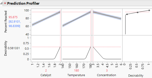
The Prediction Profiler report displays Desirability because in the Full Factorial window, you specified a Goal of Maximize when you defined your response. The desirability function shown in the rightmost cell in the top row of the profiler shows that a value of 100 is most desirable and a value of 90 or below is least desirable.
3. Click the Prediction Profiler red triangle and select Optimization and Desirability > Maximize Desirability.
Figure 13.6 Prediction Profiler Showing Settings That Optimize Desirability
The predicted mean Percent Reacted at the settings that are shown is 95.875, with a confidence interval of 92.91 to 98.84. Note that, for all three factors, the settings that are identified are at the extremes of the ranges used in the experiment. In a future experiment, you should explore the process behavior beyond these settings.


