 Example of Retaining a Factor in Generalized Regression
In this example, you construct a generalized regression model and use the active parameters to fit a reduced model. Based on this reduced model, you use the Simulate feature to explore the likelihood that one of the factors is included in the model.
A pharmaceutical manufacturer has historical information about the dissolution of a tablet inside the body and various factors that can affect the dissolution rate. A tablet with a dissolution rate below 70 is considered defective. You want to understand which factors affect dissolution rate.
Fit the Model
In this section, you fit a model using generalized regression.
Tip: If you prefer not to work through the steps in this section, click the green triangle next to the Generalized Regression script in the Tablet Production.jmp data table to obtain the model.
1. Select Help > Sample Data Folder and open Tablet Production.jmp.
2. Select Analyze > Fit Model.
3. Click Dissolution and click Y.
4. Select Mill Time through Atomizer Pressure and click Add.
5. From the Personality list, select Generalized Regression.
6. Click Run.
7. In the Model Launch panel, select the Adaptive box.
8. In the Model Launch panel, click Go.
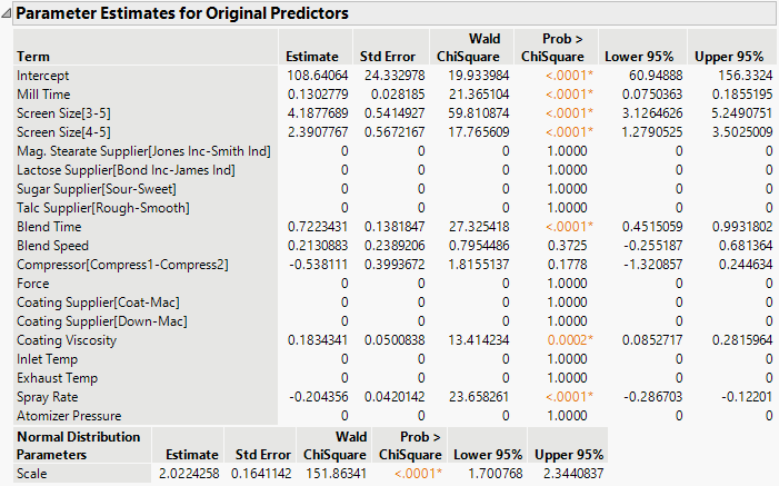
Figure 10.13 Model Based on Adaptive Lasso
You are interested in the parameter estimates shown in the Normal Adaptive Lasso with AICc Validation report. Based on the nonzero parameter estimates, the model suggests that Mill Time, Screen Size, Blend Time, Blend Speed, Compressor, Coating Viscosity, and Spray Rate are related to Dissolution.
Reduce the Model
Before reducing the model, ensure that no columns are selected in the Tablet Production.jmp data table. Selected columns are not deselected in the first step below. Ensuring that no columns are selected prevents the inadvertent inclusion of columns with zeroed terms.
If you prefer not to work through the steps in this section, click the green triangle next to the Generalized Regression Reduced Model script in the Tablet Production.jmp data table to obtain the reduced model.
1. Click the red triangle next to Normal Adaptive Lasso with AICc Validation and select Relaunch Active Set > Relaunch with Active Effects.
This opens a Fit Model window that places the terms with nonzero coefficient estimates in the Parameter Estimates reports into the Construct Model Effects list. The response is entered as Y. The Generalized Regression personality is selected.
2. Click Run.
3. In the Model Launch panel, select the Adaptive box.
4. In the Model Launch panel, click Go.
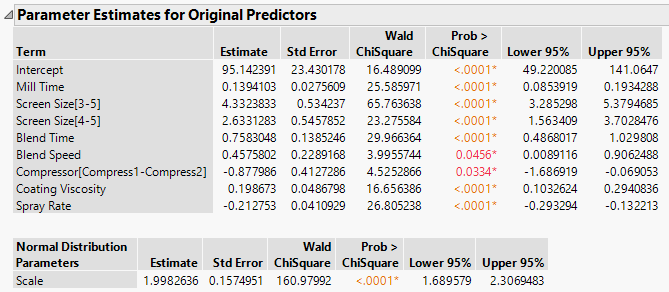
Figure 10.14 Reduced Model Using Adaptive Lasso
Notice that the estimate for Blend Speed has a confidence interval (Lower 95%) that comes very close to including zero. Next, perform a simulation study to see how often Blend Speed would be included in the model if other data values from the dissolution distribution have been observed.
Explore the Inclusion of Blend Speed in the Model
Use the report for the reduced model (Figure 10.14) in the steps below.
1. Click the red triangle next to Normal Adaptive Lasso with AICc Validation and select Save Columns > Save Simulation Formula.
This adds a new column called Dissolution Simulation Formula to the Tablet Production.jmp data table.
2. (Optional) In the data table Columns panel, click the plus sign to the right of Dissolution Simulation Formula.
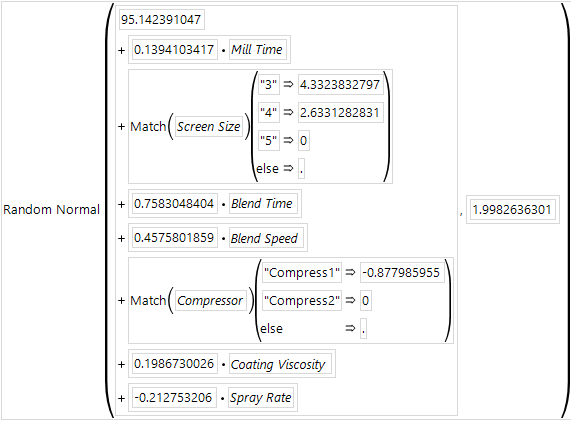
Figure 10.15 Simulation Formula
For each row, this formula simulates a value that could be obtained given the model and the distribution of Dissolution, which is estimated to be Normal with standard deviation about 1.998.
3. Click Cancel.
4. Go back to the reduced model report window. In the Parameter Estimates for Original Predictors report, right-click in the Estimate column and select Simulate.
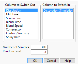
Make sure that Dissolution is selected in the Column to Switch Out list.
5. Next to Number of Samples, enter 300.
For the simulation, you ask JMP to replace the Dissolution column in each of 300 analyses with values simulated using the Dissolution Simulation Formula column.
6. (Optional) Set the Random Seed to 123.
This reproduces the values in this example.
Figure 10.16 Completed Simulation Window
7. Click OK.
The first row of the table contains the initial values of the Estimates and is excluded. The remaining rows contain simulated values.
8. Run the Distribution script.
9. Press Ctrl, click the Blend Speed red triangle and select Display Options > Customize Summary Statistics.
10. Select N Zero.
11. Click OK.
12. Scroll to the Distribution report for Blend Speed.
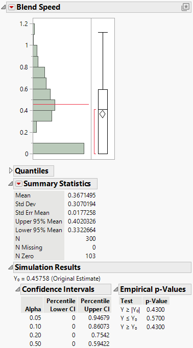
Figure 10.17 Histogram of Simulated Blend Speed Coefficient Estimates
The Summary Statistics report shows that for 103/300 = 34.3% of the simulations, the Blend Speed estimates are zero.
