Example of the Easy DOE Platform
Use the Easy DOE platform in Guided Mode to design and analyze an experiment to optimize the strength of a cup of coffee. A more complex treatment of this example using the Custom DOE platform is described in Example of a Designed Experiment in the Design of Experiments Guide.
Suppose your employer runs a medium-size coffee roasting business. You need to assess the strength of individually brewed, twelve ounce cups of coffee. Your goal is to determine how four factors impact the coffee strength and to find optimal settings for those factors.
1. Select DOE > Easy DOE.
Define
Use the Define tab to add factors and responses for the design.
Add Factors
Four factors are identified for the study: Grind, Temperature, Time, and Charge. Table 7.1 summarizes information about the factors and their settings.
|
Factor |
Role |
Range of Settings |
|---|---|---|
|
Grind |
Categorical |
Medium, Coarse |
|
Temperature |
Continuous |
195 - 205 |
|
Time |
Continuous |
3 - 4 |
|
Charge |
Continuous |
1.6 - 2.4 |
Note the following:
• Grind is a categorical factor that can take on two levels. This is also known as a qualitative factor.
• Temperature, Time, and Charge are continuous factors that can take on a numerical value. These are also known as quantitative factors.
You add the factors by factor role.
1. Note that the Factor Table has one continuous factor, you need to add two more continuous factors. Click the Add a Continuous Factor button twice.
2. Click the Add a Categorical Factor button.
Tip: You can also use the controls in the Factor Table to add factors.
Figure 7.2 Initial Factor Table on the Easy DOE Define Tab
The next steps are completed within the Factor Table. Use Table 7.1 to guide your entries.
3. Click on X1 and type Temperature. Set the value for Lower to 195, the value for Upper to 205, and the Unit to F.
4. Click on X2 type Time. Set the value for Lower to 3, the value for Upper to 4, and the Unit to min.
5. Click on X3 type Charge. Set the value for Lower to 1.6, the value for Upper to 2.4, and the Unit to q.
6. Click on X4, type Grind, change L1 to Medium and L2 to Coarse.
Figure 7.3 Completed Factor Table on the Easy DOE Define Tab
Add Response
The response is coffee Strength. It is measured as total dissolved solids, using a refractometer. The coffee is brewed using a single cup coffee dripper and measured five minutes after the liquid is released from the grounds. Previous studies indicate that a strength reading of 1.3 is most desirable, though the strength is still acceptable if it falls between 1.2 and 1.4.
1. At the top of the Define tab, click on the gray disclosure icon to open the Responses section.
2. In the Response Table, click Y under Name and type Strength.
3. Click the default Goal of Maximize and change it to Match Target. Set the Lower Limit to 1.2 and the Upper Limit to 1.4. This sets the target to 1.3.
Model
To navigate to the Model tab, either click forward on the Navigation controls at the bottom of the Define tab or click the Model tab.
Leave the Model type set to Main Effects with 12 runs. Navigate to the Design tab.
Design
The Design tab provides the design for review. At this point you run the experiment and collect the data.
Data Entry
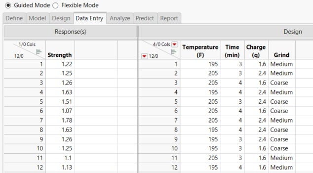
After you have run your experiment and collected data, navigate to the Data Entry tab. Enter the results of the experiment as shown below. The Easy DOE platform randomizes the run order for each design. Your design table could be in a different order than the order shown in Figure 7.4.
Figure 7.4 Strength Results
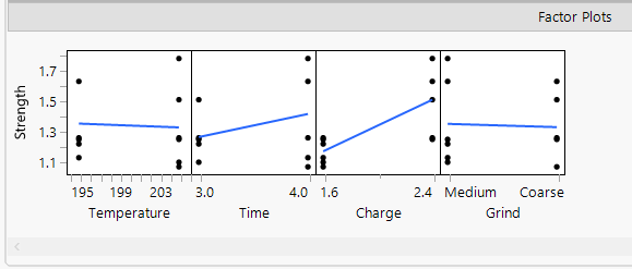
As you enter data, the Factor Plots update to show the response versus each factor. The Factor Plot shows the data points with a line connecting the mean response at each factor level. Use the plots as an initial view of which factors have the largest impact on your response. For this example, observe that Charge has the biggest impact on the Strength.
Note: The Easy DOE platform randomizes the run order for each design. Using the ordering of the responses in Figure 7.4, your results might differ from those shown in Figure 7.5, Figure 7.6, and Figure 7.9.
Figure 7.5 Factor Plots
Note: The Easy DOE platform randomizes the run order for each design. If your response ordering differs from that shown in Figure 7.4, your results might differ from those shown in Figure 7.5.
Analyze
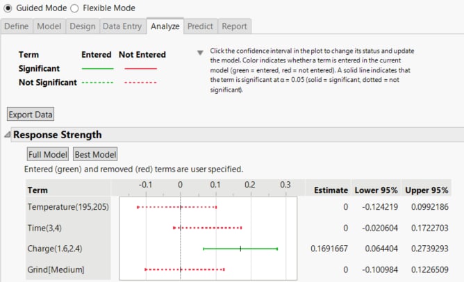
Navigate to the Analyze tab. The Response Strength report shows a plot of the estimate and 95% confidence interval for each term in your model. You are looking for terms that have a confidence interval that does not contain zero. These terms have a significant impact on the coffee strength.
You have the choice of keeping all terms in your model (Full Model), selecting the best model (Best Model), or manually selecting terms.
1. Click Best Model.
The best model has one term: Charge. The confidence intervals for Charge is colored green, which indicates that the term is in the model. The confidence interval for Charge is solid, which indicates that the coefficient is statistically different from zero at a 0.05 threshold. The confidence interval for a term that is not included in the model corresponds to the interval for the term if it were the next term entered into the model.
Figure 7.6 Analyze Tab
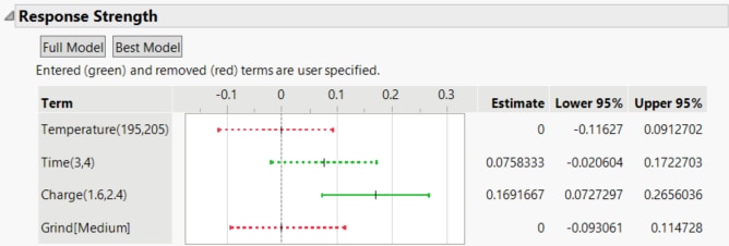
2. Click the confidence interval for Time. This enters Time into your model.
Figure 7.7 Modified Model
Time is entered into the model with a statistically insignificant coefficient. The confidence interval on the estimate of 0.07 for time includes zero, which indicates that time is not contributing to the strength.
Note: The Easy DOE platform randomizes the run order for each design. If your response ordering differs from that shown in Figure 7.4, your results might differ from those shown in Figure 7.6.
Note:
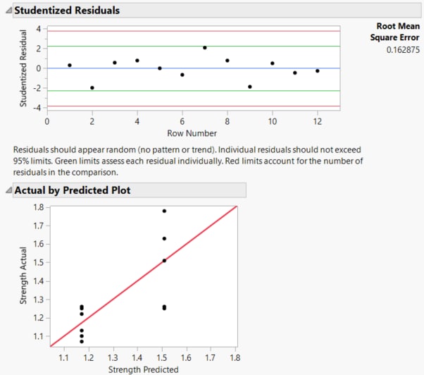
Use the Studentized Residuals plot to evaluate the model fit. All residuals fall within the green limits. The residuals do not show a pattern. You can conclude the model is reasonable. Use the Actual by Predicted plot as a second check on your model fit. The data points fall along the red Y = X line, indicating that the model predictions are reasonable.
Figure 7.8 Residuals and Actual by Predicted Plots
Note: The Easy DOE platform randomizes the run order for each design. If your response ordering differs from that shown in Figure 7.4, your results might differ from those shown in Figure 7.8.
Predict
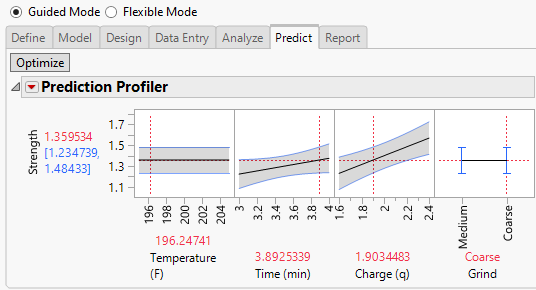
Navigate to the Predict tab and click Optimize. The optimal sets Charge to 1.9q to optimize the strength at 1.3. Note that the profiles for Temperature, Time and Grind are flat. Those factors had little impact on the strength and can be set at convenient values. Your results might show an alternative optimal solution.
Figure 7.9 Prediction Profiler on Predict Tab
Note: The Easy DOE platform randomizes the run order for each design. If your response ordering differs from that shown in Figure 7.4, your results might differ from those shown in Figure 7.9.
Report
Navigate to the Report tab. The report contains the design and analysis of your experiment. Use the Export Report button to save and share your results.


