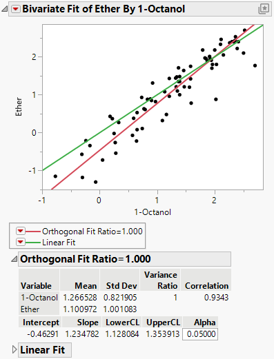
Example of the Fit Orthogonal Option
This example shows a method comparison using an orthogonal model in the Bivariate platform. One might also consider Passing-Bablok regression for comparing methods. See Passing-Bablok Fit Report. Chemical compounds were measured for solubility in different solvents.
1. Select Help > Sample Data Folder and open Solubility.jmp.
2. Select Analyze > Fit Y by X.
3. Select Ether and click Y, Response.
4. Select 1-Octanol and click X, Factor.
5. Click OK.
6. Click the Bivariate Fit red triangle and select Fit Orthogonal > Equal Variances.
7. For reference, click the Bivariate Fit red triangle and select Fit Special.
8. Select Constrain the Intercept and set to 0.
9. Select Constrain the Slope and set to 1.
This fits a Y = X line, where the intercept is 0 and the slope is 1.
10. Click OK.
Figure 5.17 Example of an Orthogonal Fit
Note that red orthogonal fit line falls below the green Y = X line for most of the data points and that the 95% confidence interval (Lower CL and UpperCL) for the slope for the orthogonal fit does not contain 1. The chemical compounds measured for solubility in Ether tend to measure lower than those measured in 1-Octanol.
