Example of the Response Limits Column Property

Use response limits to find optimal factor settings when analyzing a designed experiment. Your goal is to find factor settings that enable you to brew coffee with a target strength of 1.3, which is considered to be the most desirable value. Values less than 1.2 and greater than 1.4 are completely undesirable. The desirability of values between 1.2 and 1.4 decreases as their distance from 1.3 increases.For a complete description of the experimental design and analysis for this experiment, see Example of a Designed Experiment.

1. Select Help > Sample Data Folder and open Design Experiment/Coffee Data.jmp.

2. In the Table panel, click the green triangle next to the DOE Dialog script.

The DOE Dialog script re-runs the Custom Design that was used to create the experimental design in Coffee Data.jmp.

3. Open the Responses section.

Figure A.4 Responses in Custom Design Window 

When you designed this experiment, you specified a response Goal of Match Target with a Lower Limit of 1.2 and an Upper Limit of 1.4. Since there is only one response, you did not specify a value for Importance, because it is 1 by default. When you constructed the design table, JMP assigned the Response Limits column property to Strength.

4. Close the Custom Design window.

5. In the Coffee Data.jmp sample data table, select the Strength column and select Cols > Column Info.

6. Select Response Limits in the Column Properties list.

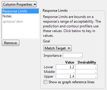
Figure A.5 Response Limits Column Property for Strength 

Notice the following:

– The Goal is set to Match Target.

– Importance is missing. When Importance is missing, JMP treats all responses in a given analysis as having equal Importance values. So JMP assigns Strength an Importance value of one.

– The Lower limit is 1.2.

– The Upper limit is 1.4.

– No Middle value is specified.

Because no Middle value is specified, the target is defined to be the midpoint of the Lower and Upper limits, which is 1.3.

– No Desirability values are specified.

7. Select the Show as Graph Reference Lines option.

This option shows horizontal reference lines for the Lower, Middle, and Upper values in the Actual by Predicted Plot and the Prediction Profiler.

8. Click OK.

9. In the Coffee Data.jmp data table, click the green triangle next to the Reduced Model script.

10. Click Run.

The Prediction Profiler appears at the bottom of the report.

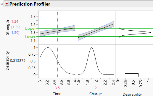
Figure A.6 Profiler Showing Desirability Function for Strength 

The desirability function for Strength appears in the plot at the right above Desirability. This plot appears because the data table contains a Response Limits column property for Strength. The Prediction Profiler also shows reference lines for the Lower and Upper limits for Strength.

11. Press Ctrl and click the Strength plot for Desirability.

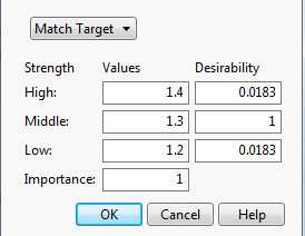
Figure A.7 Response Goal Window for Strength 

Notice the following:

– JMP determines the Middle value to be the midpoint of the High and Low limits that you specified in the Response Limits column property.

– Because the Goal is set to Match Target, JMP sets the Desirability for the Middle value to 1.

– JMP sets the Desirability for the High and Low values to very small numbers, 0.0183.

– The Desirability plot in Figure A.6 shows how JMP uses the Desirability values shown in Figure A.7. The Desirability function for Strength is essentially 0 beyond the Low and High values and it increases to 1 gradually as Strength approaches the target of 1.3. The Importance value is set to 1 since there is only one response in the model.

12. Click Cancel to exit the window.

13. Click the Prediction Profiler red triangle and select Optimization and Desirability > Maximize Desirability.

The settings for Time and Charge are updated to show settings for the factors that maximize the desirability function for Strength. However, many other settings also maximize the desirability function. SeeContour Profiler in Profilers for information about how to identify other settings that maximize the desirability function.