Example of Weibayes Analysis
The Life Distribution platform provides two possible ways to perform a Weibayes analysis:
• You have no failures (all observations are right-censored) and the preference Weibayes Only for Zero Failure Data is checked. Then the Weibayes report appears. See Weibayes Example for Data with No Failures.
• You have few failures. A full Life Distribution report is presented. Fit a Weibull distribution. In the Parametric Estimate - Weibull report, select the Fix Parameter option. Then select the Weibayes option in the Fixed Parameter report. See Weibayes Example for Data with One Failure.
Weibayes Example for Data with No Failures
You have data for a product that is mostly reliable. Thirty were tested for 1,000 hours with no failures occurring. You want to predict the failure probability at 2,000 hours.
1. Select Help > Sample Data Folder and open Reliability/Weibayes No Failures.jmp.
2. Select Analyze > Reliability and Survival > Life Distribution.
3. Select Time and click Y, Time to Event.
4. Select Censor and click Censor.
5. Select Freq and click Freq.
6. Select Likelihood as the Confidence Interval Method.
7. Click OK.
A special Life Distribution report appears. Weibayes and Weibull beta should be selected.
8. Type 1.5 as the known Weibull β value.
The value 1.5 is considered appropriate for this example.
9. Click Update.
10. In the Distribution Profiler, type 2000 for Time.
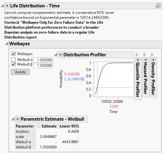
Figure 3.18 Life Distribution Report for Zero Failures
From the Distribution Profiler, you can see that at 2,000 hours, the conservative probability is 24.6058%. That means that the one-tailed conservative 95% confidence limit for the failure probability is 24.6058%.
Weibayes Example for Data with One Failure
Suppose you have the same data, but this time, one failure occurred at 800 hours. Again, you want to predict the failure probability at 2,000 hours.
1. Select Help > Sample Data Folder and open Reliability/Weibayes One Failure.jmp.
2. Select Analyze > Reliability and Survival > Life Distribution.
3. Select Time and click Y, Time to Event.
4. Select Censor and click Censor.
5. Select Freq and click Freq.
6. Select Likelihood as the Confidence Interval Method.
7. Click OK.
The Life Distribution report appears.
8. Select the Weibull distribution in the Compare Distributions plot.
9. Click the red triangle next to Parametric Estimate - Weibull and select Fix Parameter.
10. Select Weibayes and Weibull beta in the Fix Parameter report.
11. Type 1.5 as the known Weibull β value.
12. Click Update.
13. In the Distribution Profiler, type 2000 for Time.
14. Hover over the top of the Y axis. The cursor becomes a hand. Drag the axis downward until it reaches 0.5 as the top number.
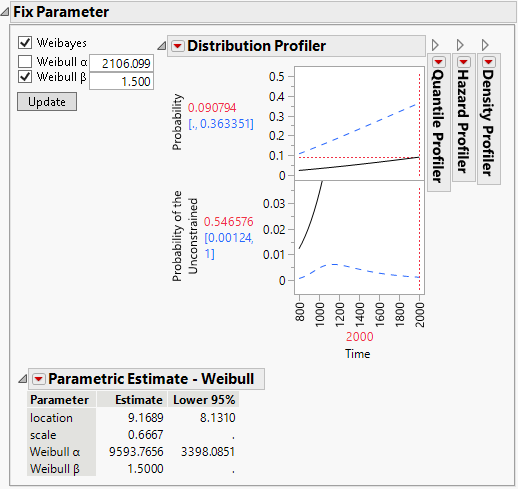
Figure 3.19 Life Distribution Report for One Failure
In the Distribution Profiler, the solid line shows the MLE. The dashed line shows the Weibayes conservative limit. You can see that at 2,000 hours, the conservative probability is 36.3351%. That means that the one-tailed conservative 95% confidence limit for the failure probability is 36.3351%.

